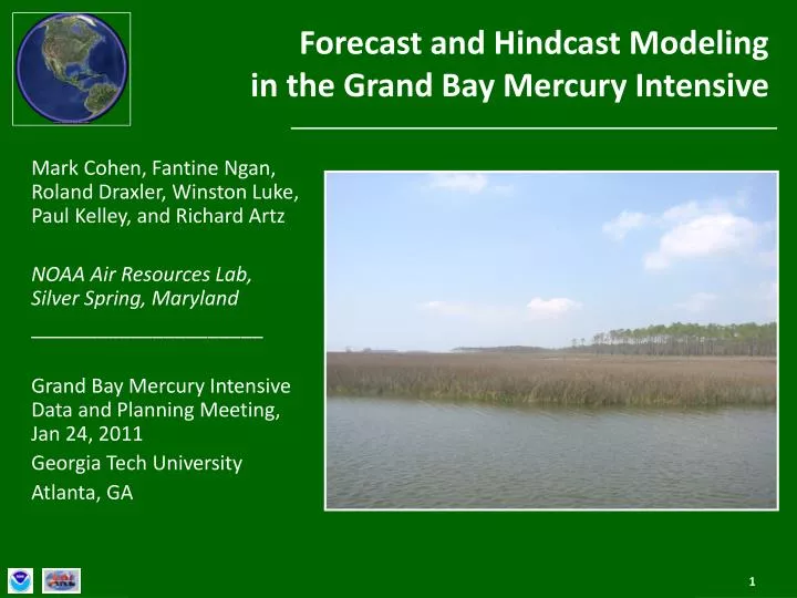
Forecast and Hindcast Modeling in the Grand Bay Mercury Intensive

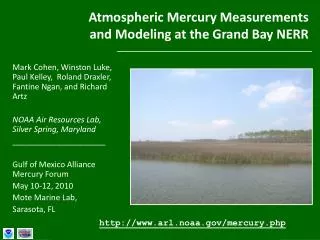
1. Forecast and Hindcast Modeling in the Grand Bay Mercury Intensive Mark Cohen, FantineNgan, Roland Draxler, Winston Luke, Paul Kelley, and Richard Artz NOAA Air Resources Lab, Silver Spring, Maryland _____________________ Grand Bay Mercury Intensive Data and Planning Meeting, Jan 24, 2011 Georgia Tech University Atlanta, GA

2. Outline • Forecasting for mission planning • High-resolution hindcast meteorological modeling (FantineNgan) • Atmospheric Mercury and Other Hindcast Modeling Hg from other sources: local, regional & more distant emissions of Hg(0), Hg(II), Hg(p) Reactive halogens in marine boundary layer Measurement of ambient air concentrations • Enhanced oxidation of Hg(0) to RGM? • Enhanced deposition? Measurement of wet deposition wet and dry deposition to the watershed wet and dry deposition to the water surface

3. Forecasting for Mission Planning During the Summer 2010 Intensive • Based on the NOAA NCEP NAM 12km weather forecast model product • This forecast starts at UTC 00 for the given date, which is 7 PM the night before in Grand Bay time (GBT). • The hours displayed in the product – 9 AM to 8 PM GBT – thus represented hours 14-25 in the 48 hr t00z forecast. • The file became available to NOAA ARL at ~2:00 AM GBT, and the processing of the data to make this product was generally done by 5:00 – 6 00 GBT. • Goal was to have product ready each day by 7:00 GBT

4. Based on the t00z NAM-12km forecast generated by the National Weather Service HYSPLIT-based forecast product for the Grand Bay Intensive • Meteorological Data Contours(pages 26-37) • One page for each local hour from 9 AM to 8 PM • Image in upper left corner and upper middle are the mixing height (same map as shown on Trajectory pages). The two maps are slightly different due do differing interpolation procedures • The map in the upper right corner is forecast precipitation, shown as a 3-hr accumulation, ending at that hour; that is the amounts shown are the total forecast precipitation over the previous 3 hrs. • Other maps shown are for the following three surface parameters: pressure, downward shortwave radiation flux, and friction velocity This forecast starts at UTC 00 for the given date, which is 7 PM the night before in Grand Bay time (GBT). The hours displayed in this product – 9 AM to 8 PM GBT – thus represent hours 14-25 in the 48 hr t00z forecast. The file becomes available to NOAA ARL at ~2:00 AM GBT, and the processing of the data to make this product is generally done by 5:00 – 6 00 GBT. • Trajectories(pages 2-13) • One page for each local hour from 9 AM to 8 PM • Image in upper left corner is mixing height (m) • The other five images are back-trajectory maps, each map representing a starting point at a different elevation (meters) above mean-sea-level (250, 500, 1000, 2000, and 3000) • There are nine trajectories shown on each map: one starting at the Grand Bay NERR and on a +/- 1 deg lat/long grid around the NERR • The trajectories each go back 96 hours; but the trajectories may not stay on the map for all 96 hours. • On each trajectory there is a little dot showing the location at six-hour intervals; and a larger symbol at 00 UTC each day. • In the panel below the trajectories, the height above the surface is shown for each trajectory as it goes back in time • Note that elevations in trajectory maps are shown as being “above ground level”, and the starting heights labels in the panels below each trajectory are shown for the first trajectory run. This happened to started over land where the elevation was ~80m, so, the labels happen to refer to that trajectory, so the labels say ~170, 420, 920, 1920, and 2920. • Meteorological Data for Grand Bay NERR(pages 38-50) • Page 38 is description of data that are shown • Then, one page for each local hour from 9 AM to 8 PM • Each page shows the meteorological data at the surface and at each level of the gridded, forecast meteorological data set. • Note that on these pages and throughout, times are expressed in UTC (Universal Time Coordinate). These are currently 5 hrs ahead of Grand Bay, e.g., 9 AM Grand Bay is 2 PM UTC (or UTC 14) • RGM Plumes from Large Regional Sources(pages 51-63) • Page 51 shows a map of some of the large sources in the region; as stated on map, some of the sources are no longer emitting. These sources were not included in these simulations. • One page for each local hour from 9 AM to 8 PM; each page shows model-estimated RGM concentrations for six different vertical layers n the atmosphere. • These maps do not represent the total RGM in the atmosphere, but only the fraction contributed by large regional sources. • The maps show average concentrations for the hour leading up to the stated hour, e.g., the map for UTC 14 represents average concentrations between UTC 13 and 14 (8 – 9 AM Grand Bay) • Wind Direction at Different Elevations(pages 14-25) • One page for each local hour from 9 AM to 8 PM • Each image shows a map of wind direction, at each grid point in the NAMSF 12-km forecast at a particular vertical level in the met data set • There are 6 maps, corresponding approximately to the elevations 10, 250, 500, 1000, 2000, 3000. • The met data is on “terrain following sigma levels”; so, the heights above the ground at any given location are influenced by the terrain height.

5. The first set of pages were hourly maps of mixing heights and back trajectories

7. 7

9. The second set of pages were hourly maps of wind vectors at different heights

13. The third set of pages were hourly maps of mixing height, PBL-height, 3-hr precipitation, surface pressure, downward shortwave radiation flux and friction velocity

26. The fourth set of pages were hourly tables of surface variables and meteorological parameters in a vertical column above the site

31. The fifth set of pages were hourly maps of modeled RGM concentrations in the region, arising from anthropogenic sources in the region

44. Forecasting for next intensive? • What format would be most helpful? • Maybe just have one page per hour, and then one could look at one part of the page as one scrolled through… • This would mean far less information, though, as we are limited to about six images per page… • If we did it this way, what would the six images be? • Or maybe this is too limited? • Another issue was bandwidth for downloading – I had to degrade the quality of the images significantly in order to keep file size as small as it was (~12 MB), and even this was perhaps too large

46. 2. High Resolution HindcastMeteorological Modeling A 4-km meteorological data modeling analysis (with data assimilation) has been produced by Dr. FantineNgan, a post-doc at NOAA ARL, for the Summer 2010 Intensive Unfortunately, Fantine couldn’t be at this meeting as she is at the AMS meeting in Seattle this week, but she prepared the slides in this section for presentation here 10 m wind fields 18 UTC August 06

47. Domain configuration Projection center: 40N, 100W Standard latitude: 30N, 60N Layers: 43, with model top at 50 mb (1st layer thickness is 33 m and 15 layers are below 850 mb) D01 D02 D03 Grand Bay – 30.4123, -88.4037, 5 m

48. Model Setup Simulation period: 210/07/31 00 UTC – 08/13 12 UTC IC/BC for D01 is from GFS data + objectively analysis (OBS2GRID) Others are nestdown from coarse domain. 3D grid nudging, SFC nudging and OBS nudging are on for all domains The model was run in 5.5 day segments and re-initialized every 5 days. There were 12 hours overlapping between each run segment. The soil moisture and temperature in the input files were replaced with the WRF output in the previous run segment run segment period p1 7/30 00 UTC – 8/4 12 UTC p2 8/4 00 UTC – 8/9 12 UTC p3 8/9 00 UTC – 8/13 12 UTC Physical options microphysics: WSM 3-class scheme radiation scheme: RRTM scheme for longwave radiation Dudhia scheme for shortwave radiation land surface model: PX LSM PBL scheme: ACM2 scheme cumulus scheme: Grell-Devenyi Ensemble scheme

49. Temperature time series at Grand Bay Black *: observation, Red line: WRF model Relative humidity time series at Grand Bay • Measurements are provided by Winston Luke

50. Wind speed time series at Grand Bay Black *: observation, Red line: WRF model Wind direction time series at Grand Bay