Download
1 / 22
220 likes | 394 Views
Toward Forecasting Space Weather. Tamas Gombosi The University of Michigan Isradynamics 2010 Conference Ein Bokek (Dead Sea), Israel April 11-16, 2010. Space Weather.

E N D
Toward Forecasting Space Weather Tamas Gombosi The University of Michigan Isradynamics 2010 Conference EinBokek (Dead Sea), Israel April 11-16, 2010
Space Weather Space weather: conditions in geospace that can have adverse effects on space-borne and ground-based technological systems and can endanger human life or health. (courtesy of Doug Biesecker, NOAA SWPC)
Modeling the Space Weather System Disparate time scales Disparate spatial scales Disparate physics …… ☞ Model coupling is needed
Coupled Space Weather Models • Space Weather Modeling Framework (SWMF) • Centered at the University of Michigan • Enables flexible Sun-to-Earth model chain • Single executable • Center for Integrated Space Weather Modeling (CISM) coupled model • Centered at Boston University • Enables Sun-to-Earth model chain • Multiple executables • Integrated Magnetosphere-Ionosphere Model • Centered at the University of New Hampshire • Couples a global magnetosphere, an ionosphere-thermosphere, a radiation belt and a ring current model • Single executable
SWMF Capabilities: Physics Fluid Equations Additional Physics Multiple materials Non-ideal EOS Radiation Gray diffusion Multigroup diffusion Source terms Gravity, mass loading, chemistry, photo-ionization, recombination, etc… Various resistivity models Semi-empirical coronal heating Alfven wave energy transport and dissipation Self-consistent turbulence • Compressible HD • Ideal MHD • Semi-relativistic MHD • Resistive MHD • Single-fluid Hall MHD • Two-fluid Hall MHD • Multi-species (Hall) MHD • Multi-fluid (Hall) MHD • Anisotropic pressure • Heat conduction
SWMF Capabilities: Numerics • Time integration Schemes • Local time-stepping for steady state • Explicit (with Boris correction) • Explicit/implicit • Semi-implicit • Point-implicit • Grids • Block-adaptive tree • Cartesian • Generalized grids including spherical, cylindrical, toroidal • TVD Solvers • Roe • HLLD • HLLE • Artificial-wind • Rusanov • Limiters • Koren (3rd order) • MC • Beta • Div(B) control • 8-wave • Hyperbolic/parabolic scheme • Projection • Staggered grid (CT) • Ray tracing • Fast & parallel • Synthetic images • White light coronagraph • EUV LOS • 171Å, 195Å, 284Å • X-ray radiographs • Tomography
SWMF Capabilities: Framework • Source code: • 250,000 lines of Fortran in the currently used models • 34,000 lines of Fortran 90 in the core of the SWMF • 13,000 lines of Fortran 90 in the wrappers and couplers • User manual with example runs and full documentation of input parameters • Fully automated nightly testing on 9 different machine/compiler combinations • SWMF runs on any Unix/Linux based system with a Fortran 90 compiler, MPI library, and Perl interpreter
Simulation and Tomography ne=106 ne=5x10⁵ 2005 05 14 21:03 2005 05 15 21:05 2005 05 16 21:00 2005 05 17 21:05 2005 05 18 21:00 2005 05 19 21:05 2005 05 20 21:00 2005 05 21 0306 Frazin et al., 2008 2005 05 21 21:05 2005 05 22 21:05 2005 05 23 21:00 2005 05 24 21:05 2005 05 25 21:00 2005 05 26 21:05 2005 05 27 21:00 2005 05 27 23:44
Thermodynamic Solar Wind Model(van derHolst, Oran and Sokolov) • Sub-photosphere model • Multigroup radiation transport • MHD • Magnetic flux emergence • Low corona (1R☉r<2.5 R☉) • γ=5/3, single temperature • Heat conduction • Transport and dissipation of total energy of Alfvénic turbulence (E±) • Wave dissipation represents sources for the plasma momentum and internal energy • Additional coronal heating is obtained from the “unsigned flux” model (Abbett 2007) and observed X-ray luminosity (Pevtsov 2003) • Corona (2.5R☉<r<20R☉) • γ=5/3, separate ion and electron temperatures • Transport and dissipation of frequency resolved Alfvén wave intensity, I±(ω) • Kolmogorov spectrum is assumed at the inner boundary • Observational inputs: • Magnetogram driven potential field extrapolation (synoptic maps from GONG or MDI) • Density and temperatures near the sun are predicted by the DEMT (Differential Emission Measure Tomography) results of Vasquez and Frazin (2009). • Solar X-ray luminosity (EIT, STEREO)
Boundary Conditions for CR2077with no Free Parameters GONG magnetogram WSA relation STEREO/EUVI Differential Emission Measure Tomography (Vasques & Frazin)
CR2077: Two State Solar Wind Radial velocity • In the fast wind • Electrons are cold (due to adiabatic cooling) • Ions are hot (due to Alfvén wave heating) • In the slow wind • Electrons are hot (due to heat conduction) • Ions are cold (no Alfvén wave heating) Ion temperature Electron temperature
New Low Corona Model EIT 171Å EIT 195Å EIT 284Å SXT AlMg CR1913 Old SC model synthesis New LC model synthesis Observation: Aug 27, 1997 Downs et al., ApJ, 712, 1219, 2010
Alfvénic Turbulence and SEP Acceleration t=7m t=80m t=137m • Recent Hinode observations imply that MHD turbulence might be the source that powers, accelerates and heats the solar wind • Today it is possible to use many dimensional models (>3D) • We developed a coupled solar wind-turbulence-SEP model • Separate transport equation is solved for turbulence • Wave stress tensor and energy appear in the solar wind momentum and energy equations • Energetic particles are accelerated by interaction with turbulence Sokolov et al., 2009
FTE Simulation (Kuznetsova) • Resolution at the dayside magnetoapuse is 1/16 RE (400 km) • Total number of cells in the simulation is 20 million • Solar wind parameters: • n = 2 cm–3 • T = 20,000 K • Vx = 300 km/s • B = 5 nT • IMF Turning From Northward (θ = 0∘) to IMF clock angle θ < 120∘
Theta = 120o Subsolar FTE Structure Cluster Pressure
View from the Sun Component Reconnection Near Sub-Solar Region (Y ~ 0 – 2 RE) And Anti-Parallel Reconnection at Flanks (Y ~ 12 - 15 RE)
X-slice Y-slice Z-slice FTE at flanks (Y = 12 Re) is connected to FTE at the subsolar region ( Y = 0 ).