Download
1 / 71
1.18k likes | 1.81k Views
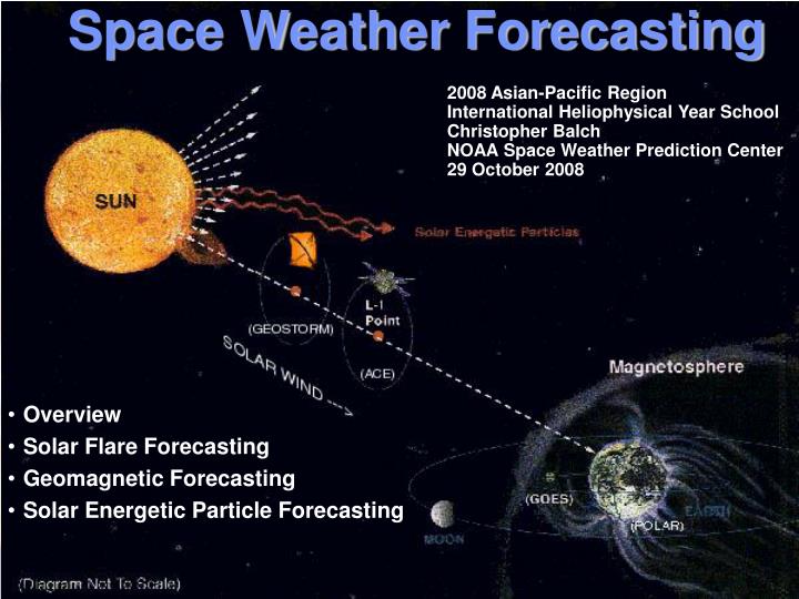
Space Weather Forecasting. 2008 Asian-Pacific Region International Heliophysical Year School Christopher Balch NOAA Space Weather Prediction Center 29 October 2008. Overview Solar Flare Forecasting Geomagnetic Forecasting Solar Energetic Particle Forecasting. General Points.

E N D
Space Weather Forecasting 2008 Asian-Pacific Region International Heliophysical Year SchoolChristopher BalchNOAA Space Weather Prediction Center29 October 2008 • Overview • Solar Flare Forecasting • Geomagnetic Forecasting • Solar Energetic Particle Forecasting
General Points • Physical Models have not developed to the point of being useful operationally • There are efforts to improve this situation • Center for Integrated Space weather Modeling (CISM) • Coordinated Community Modeling Center (CCMC) • Center for Space Environment Modeling(CSEM at University of Michigan)
Forecasting Today • Key inputs • Conceptual models • Observational data • Empirical models • Much depends on the human forecaster to analyze and synthesize the information
I’m going to need those… Forecaster From www.explodingdog.com Forecaster Brains
The Weather Analysis and Forecasting Process • What happened? • Why did it happen? • What is happening? • Why is it happening? • What is going to happen? • Why is it going to happen? • How did/is/will it affect(ing) my customers? Diagnosis Nowcasting Prognosis - Forecasting Bosart, 2002
Types of Forecasters • Intuitive Scientists • Rules-Based Scientists • Procedure-Based Observers • Procedure-Based Mechanics • Disengaged Pliske et. al., 1997
maintain situational awareness are organized and can multitask deal well with pressure are decisive are flexible develop good visualization and conceptualization skills are passionate about [their work] are able to deal with failure are continuous learners have good “people” skills have good communication skills can adapt to shift work Good Forecasters… Doswell, 2003
cultivate increasing technical proficiency synthesize knowledge into useful wx info recognize customers needs, knowledge level and expectations learn from peers & past events distinguish between mechanical and diagnostic prowess are interested and passionate about [their work] – professionally dedicated have good management/people skills (delegation, prioritization, mentoring) acknowledge other perspectives and can tolerate criticism/disagreement are honest & accountable maintain a productive rapport with researchers / modelers scrutinize model output have stamina for shift work Good Forecasters… Stuart et. al., 2006
Challenges • Time pressure • Too much, too little, bad or conflicting data • Conflicting, or bad model output • Incomplete conceptual models • Human Factors (IT, Rust, Policy, Staffing, Face-Threat)
Key Data Sources • Ground Sites • Magnetometers (NOAA/USGS) • Thule Riometer and Neutron monitor (USAF) • SOON Sites (USAF) • RSTN (USAF) • Telescopes and Magnetographs • Ionosondes (AF, ISES, …) • GPS (CORS) • SOHO (ESA/NASA) • Solar EUV Images • Solar Corona (CMEs) ESA/NASASOHO • ACE (NASA) • Solar wind speed, density, temperature and energetic particles • Vector Magnetic field L1 NASAACE NOAA GOES NOAA POES • STEREO (NASA) • Solar EUV Images • Solar Corona & Heliosphere (CMEs) • In-situ plasma & fields • In-situ energetic particles • SWAVES • GOES (NOAA) • Energetic Particles • Magnetic Field • Solar X-ray Flux • Solar EUV Flux • Solar X-Ray Images • POES (NOAA) • High Energy Particles • Total Energy Deposition • Solar UV Flux
Solar flares • What is a solar flare ? • H-alpha classification system • X-ray classification system June 6, 2000 at 1616 UTC Holloman Solar Observatory June 6, 2000 at 1715 UTC SXT GOES XRS 5-7 June 2000
H-alpha flare classification system • Two letter classification based on H-alpha • Importance: based on area of brightening • Brightness: Line width of intensity increase • Example: 1B means area of 100-250, brightness such that ≥20 millionths is at ≥ 50 % above bkgnd± 1.0 Å of H-alpha center
X-ray flare classification system • Based on total (spatially integrated) x-ray flux from Sun in 1-8 Å band • Continuous observations provided by GOES satellites • Letter, number system: letter for ‘decade’, number for level in decade Example:if peak flux is 2.3 x 10⁻⁵ then x-ray class is M2.3
Solar Active Regions and Flare Prediction • C, M, X, Proton probabilities 1-3 days • Images used: white light, surface magnetic fields, H-alpha, X-ray • Focused on active regions and magnetic field structure • Baseline – climatology • Persistence June 5, 2000 at 1714 UTCBig Bear Solar Observatory Analysis • Why is a given region flaring ? • Evaluate complexity, dynamics, rate of growth/decay, ‘hot spots’ • Looking for shear, proper motion, differential rotation effects • E/W vs N/S inversion lines June 7, 2000 at 1430 UTCMt Wilson Solar Observatory
Solar magnetic field • Sunspots and magnetic fields • Observations • Magnetic classification system • Vector magnetic fields • Conceptual model for magnetic loops • ‘Potential fields’ • ‘Non-potential’ fields • Relationship to flare probability • Role of growth, decay, differential rotation, proper motions
Extension of magnetic fields into the corona Storing energy in the coronal magnetic field
Flare Prediction Tool Forecaster- entered values Forecast these values using the formula RTOTAL = 1-[(1-R1) *(1-R2)*… *(1-Rn )] where R1, R2 ,… ,Rn are C, M or X flare probabilities for the individual regions on the disk. Statistical probabilities Observed flares
Limitations • Usually do not have vector field observations • No one really knows what triggers a flare • Concept of self-organized criticality • Do not know when new flux will emerge or old flux will decay • No physical model guidance
Developmental Activitiesthat may improve flare forecasting • Helicity as a driver of eruptive events • Parameters derived from vector magnetograms • Also exist studies deriving parameters from line-of-sight magnetograms • Bayesian methods to combine multiple inputs (e.g. persistence and sunspot classification) • Solar dynamics observatory • Helioseismology (to detect emerging flux…)
Geomagnetic Forecasting • Physical Drivers of Geomagnetic Activity • Transients from CME’s • Recurrent High Speed Streams from Coronal Holes • Additional Factors to consider • Seasonal effects (climatology) • Continuation of current levels (persistence)
Geomagnetic Specification Using Indices • A summary of activity: • The indices are intended to provide a summary of variations of the Earth’s magnetic fields • An interpretation: • Helps to extract a particular type of magnetic variation or an ensemble of variations (as related to one or more magnetospheric or ionospheric current systems) • Help users and non-specialists • Enable users to distinguish between times of high risk and low risk • Non-specialists can know the the ‘level’ of activity without having to interpret magnetograms or satellite data • Facilitate comparative studies • Compare activity level with related phenomena • Study cause-effect relationships • Investigate long time series behavoir • Simplify predictions of activity levels which are based on solar or solar wind observations
K-index & A-index • Measure of 3 hourly range of irregular variations: • Designed for sub-auroral and mid-latitude stations • Time interval optimized for 45-180 minute timescales: • magnetic bays – typical signature of an electrojet injection • Subtraction of SR:daily regular variation from the magnetometer data • Maximum of range of horizontal components: • scaled from 0 to 9 using quasi-log scale (e.g. from Boulder): Range: 0-4 5-9 10-19 20-39 40-69 70-119 120-199 200-329 330-499 500 K: 0 1 2 3 4 5 6 7 8 9 • Normalization by geomagnetic latitude: (e.g. K9 threshold in Boulder is 500, College is 2500), to get similar K frequency distributions • K9 occurs about 0.1% of the time (~30 times per solar cycle) • 24 hour A-index – average of 3-hourly equivalent amplitutes, ak: K 0 1 2 3 4 5 6 7 8 9 ak 0 3 7 15 27 48 80 140 240 400
Planetary Kp/Ap • Kp: a type of planetary average of station K-indices • A specific set of sub-auroral stations is used • The calculation includes a ‘standardization’ for each station K-index • Kp is discretized into 28 levels from 0 to 9 • Kp-est: USAF estimate of Kp based on real-time data • Different observatory network • Network has a Northern American bias • Currently updated on one-hour cadence • Ap/Ap-est: 24 hourly index of activity • Calculated just like the 24-hour A-index for a single station • Based on Kp/Kp-est
Activity Categories • Qualitative activity level descriptor based on K & A
Geomagnetic Forecasts Sources: • Earthward-directed CME’s • Coronal-hole high speed streams Prediction inputs – CME’s • CME properties • Properties of associated x-ray event • Location of associated activity • Radio signatures (Type II/Type IV) • Medium energy particles (ACE) Prediction inputs – CH’s • Size & Location or CH • Polarity of CH • Comparison with previous rotation
Solar Wind & Coronal Holes • Open field regions • Source of high speed solar wind • High Speed Stream (HSS) • Evolve slowly from rotation to rotation • Plasma characteristics: • elevated T • low density • presence of Alfven waves
Solar Wind & Coronal Holes • Co-rotating Interaction Region (CIR) • The HSS builds up a leading CIR • Plasma characteristics: • Compressed • Enhanced Density • Enhanced Magnetic Field • Possible shock formation • In some cases the CIR shock will accelerate particles • Solar wind signatures look similar to a transient
Recent 27 day plot of solar wind data, showing the high-speed stream structure
Russell McPherron Effect Long-known semi-annual variation of geomagnetic activity Svalgaard et al, 2002 A spiral field will have components Bx and By in the solar-equatorial coordinate system (GSEQ) The Solar Magnetospheric coordinate system is rotated about X, so the By component in GSEQ will have By and Bz components in GSM (e.g. the Earth’s ‘dipole’ tilts into or away from the spiral field) Away sector more geoeffective in fallTowards sector more geoeffective in spring Russell & McPherron 1973
Coronal Hole Forecasting • Recurrence – what happened 27 days ago? • Recurrence can help to identify co-rotating disturbances; the best view is obtained by looking at a 27 day plot of solar wind data • Look for changes in coronal hole morphology for this rotation relative to last rotation – this should be factored in as a small modification to recurrence • Remember semi-annual variation of geomag activity • Positive holes are more geoeffective in the fall, negative holes are more geoeffective in the spring • CIR’s lead coronal holes and can look similar to CME’s (Temperature provides the key clue)
Coronal Hole Forecasting Challenges • Timing can be difficult • Depends on SW speed • Coronal hole boundaries don’t provide full information about expansion in the heliosphere • Evolution is slow but occurs • Can miss timing by 12-24 hours easily
Coronal Hole Forecasting Challenges • Timing can be difficult • Depends on SW speed • Coronal hole boundaries don’t provide full information about expansion in the heliosphere • Evolution is slow but occurs • Can miss timing by 12-24 hours easily • Stereo-B can help • There are subtle effects in addition to co-rotation that have to be accounted for
Solar Wind - Transients • Coronagraph data are critical • POS speed can be estimated • lower constraint on transit time • Interaction of CME with ambient solar wind is important • Back-to-back CME’s – second CME won’t slow down very much • Size of CME as it moves out is difficult to know
Solar Wind - Transients • CME’s in the solar wind • Shock, sheath, driver • Transit times for CMEs • Using EPAM ENLIL model HAF model
Geomagnetic Forecasting: Transients • CME-driven disturbances • As the CME moves out it develops three key components: shock, sheath (swept up solar wind), and driver (simple conceptual picture) • What direction is CME going, how fast, what kind of solar wind is it ‘plowing’ through ? • Will Earth go through the center, through the side, maybe we will only go through the sheath, or maybe it will miss earth altogether • Have to rely on grey-matter fusion to estimate CME trajectory: use location on disk and visual appearance • STEREO –it will help although we don’t have an objective technique at this point
Example: X3/4B flare with CME Fast moving CME, estimated POS velocity 1500 km/s d/v calculation ~ 28 hours
Response to X3/CME at 13/0240Z - ~35 hour transit time Sheath Driver/Cloud Shock at 14/1356Z
Geomagnetic Forecasting: Transients • CME-driven disturbances • EPAM also provides clues (Energetic Particles on ACE) • Absence of EPAM signatures is a decent indicator that we won’t get hit, at least not by a strong CME • Timing: distance/velocity provides a lower limit on the arrival time (the fast CME’s tend to decelerate). However, if the solar wind has been previously swept up by a preceding CME, deceleration of the successive CME is usually small • For earthbound CME’s, speed is probably the best indicator of storm severity
ACE EPAM shows rise in flux ahead of the interplanetary shock
Limitations • Arrival time is the biggest challenge today • Must somehow account for the swept up component of the solar wind • Geometry of the shock, the sheath, and the driver are all uncertain • Magnetic field in the driver is unknown • Not obvious if it can be determined w/o in-situ measurements
Solar Energetic Particles:nowcasts, forecasts, products • GOES real-time particle flux data • Range of energies 0.6 – 500 MeV • Event defined as flux of 10 p cm-2 s-1 ster-1 (PFU) at > 10 MeV • Daily forecast • Three day probabilities for SEP events • Short term warnings • Based primarily on flare observations • Thresholds: 10 PFU 10 MeV and 1 PFU 100 MeV • Prediction for onset time, maximum flux, time of maximum flux, and expected event duration • Alerts • Real-time reports of an observed event • Issued shortly after threshold has been attained • Additional notices at 100, 1000, and 10000 PFU. • Event Summaries • Important for users to have an ‘all-clear’ indicator
Reames, 1999 Solar Energetic Particle Event Forecasting Sources: • Strong CME-driven shocks • Energetic flares in active regions Available Prediction Inputs • X-ray maximum and integral flux • Location of associated activity • Radio signatures (Type II/Type IV) • CME properties (speed, total mass, direction) Cane et al, 1988
Measuring SEPs GOES Energetic Particle Sensor (EPS) Monitors the energetic electron, proton, and alpha particle fluxes e: 0.6 to 4.0 MeV p: 0.7 to 700 MeV a: 4 to 3400 MeV SWPC processes the data to derive integral proton fluxes: ≥ 10 MeV ≥ 30 MeV≥ 60 MeV ≥ 100 MeV Proton Event defined: ≥ 10 PFU ≥ 10 MeV
Energetic Storm Particles (ESP) • Prior to shock passage:particle trapping leads to flat time-intensity profiles at lower energies due to streaming limit • Leads to “Energetic Storm Particles” (ESP) when shock passes the Earth • Leads to a ‘broken-power law’ energy spectrum • Even high energy particles can be trapped in the big events
SEP forecasts • Three day prediction • Starts with the flare prediction • Factor in location of the region (west is better) • Factor in age of the region (older is better) • Include persistence of ongoing events • Warnings • Key inputs: Integrated x-ray flux, type IV, type II, location, CME speed • Longitude/spectrum dependence • Statistical guidance available but has its limits • If a Earthbound CME is associated there is a possibility for an ESP event • History of the active region • Comparison with past, similar events