Download
1 / 25
250 likes | 415 Views
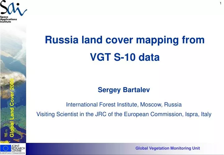
Russia land cover mapping from VGT S-10 data. Global Land Cover 2000. Sergey Bartalev International Forest Institute, Moscow, Russia Visiting Scientist in the JRC of the European Commission, Ispra, Italy. Global Vegetation Monitoring Unit.

E N D
Russia land cover mapping from VGT S-10 data Global Land Cover 2000 Sergey Bartalev International Forest Institute, Moscow, Russia Visiting Scientist in the JRC of the European Commission, Ispra, Italy Global Vegetation Monitoring Unit
Geographical extent of the study and used SPOT4-VGT data Global Land Cover 2000 Type of products used : SPOT 4-VGT S10 products including spectral and angular data Geographical extent :420N - 750N and 50E -1800Ewith particular attention to Russian territory and the boreal zone of Eurasia Time window : from end of March 1999 until beginning of November 1999 Global Vegetation Monitoring Unit
Distribution of the forest in the World Global Land Cover 2000 Boreal and Temperate Zone World Global Vegetation Monitoring Unit
The key elements being taken into consideration to design the land cover mapping method • requirements of users and particularly at national level • the satellite data properties allow to distinguish the land cover types • regional environment peculiar properties • availability of auxiliary (non satellite) data • practical realizability due to existing technical and other limitation Global Land Cover 2000 Global Vegetation Monitoring Unit
The main options and obstacles to classify the land cover types with SPOT4-VGT data Options: • spectral properties the land cover types • spectral-phenological changes of the land cover • the angular anisotropy of reflected radiation of land cover Obstacles: • presents of the pixels contaminated by clouds/shadow and snow • presents of the pixels contaminated MIR defective detectors • Sun/View directional dependence of spectral response • dependence of phenological changes both from time of observation and geographical location Global Land Cover 2000 Global Vegetation Monitoring Unit
OPTIONS OBSTACLES Spectral-Phenological features Spectral-Angular features (BRDF) Sun/View directional dependence Phenological changes Relation between main options and obstacles to classify the land cover types with SPOT4-VGT data Spectral features (single image) Global Land Cover 2000 Contamination by clouds, snow and MIR defective detectors Global Vegetation Monitoring Unit
NIR GLADES NIR HAYFIELDS GLADES CUTTINGS HAYFIELDS BOGS CLOSED SCARS STANDS BOGS SETTLMENTS PASTURE SETTLMENTS SCARS CUTTINGS PASTURE CLOSED STANDS WATER WATER MIR RED Separability of main land cover types with spectral signatures derived from single S-10 SPOT4-VGT image Global Land Cover 2000 Global Vegetation Monitoring Unit
NIR NIR DAMAGED FIR BIRCH BIRCH ASPEN PINE ASPEN FIR PINE FIR DAMAGED FIR MIR RED Separability of different species forest with spectral signatures derived from single S-10 SPOT4-VGT image Global Land Cover 2000 Global Vegetation Monitoring Unit
Steps of the satellite data pre-processing • Producing the mask of contaminated pixels related to snow, clouds and MIR channel defective detectors with the following steps procedure: • detection of utterly contaminated pixels with pre-specified thresholds • detection of “slightly” contaminated pixels with pixel-by-pixel adaptive thresholds derived from time series of data • “Hot-spot” factor normalization of spectral reflectance with BRDF model (subsidiary andoptional step) • Producing the seasonally optimised composites of spectral channels • Producing of the spectral-angular parameters with two options are considered: • statistics of Sun-Earth-Sensor relative angular parameters derived under condition of maximum NDVI pixels selection • BRDF model derived parameters estimation Global Land Cover 2000 Global Vegetation Monitoring Unit
Clouds and Snow spectral properties. Normalised Different Snow Indexes NDSI Global Land Cover 2000 NDSI = (CH1-CH4) / (CH1+CH4) From Hall et al., 1998: "Algorithm Theoretical Basis Document (ATBD) for the MODIS Snow-, Lake Ice- and Sea Ice-Mapping Algorithms. Version 4.0" Global Vegetation Monitoring Unit
Detection of the contaminated pixels Step 1: Detection of the pixels utterly contaminated by snow and clouds with pre-specified thresholds • Snow/Ice: Cs (, t*) = 1 R1 (, t*) >= 0.1 AND NDSI (, t*) >= 0.1 • Clouds: Cc (, t*) = 1 R1 (, t*) >= 0.1 AND - 0.1 < NDSI (, t*) < 0.1 • where • - geographical co-ordinates; t* - fixed time of observation (decade); • Ri ( i=14) - reflectance in the channel i ; NDSI - snow indexes; • Cs- set of snow detected pixels ; Cc- set of clouds detected pixels ; • {CP1} {Cs}U {Cc} - set of contaminated pixels at the 1st step Steps 2J: Detection of the defective detectors and “slightly” contaminated by snow/clouds pixels with adaptive thresholds derived from time series of data CP'j(*, t)= 1 t R4 (*, t) Mj (R4 (*) CPj-1(*, t) 1) + 2SDj (R4 (*) CPj-1(*, t) 1) OR R4 (*, t) Mj (R4 (*) CPj-1(*, t) 1) - 2SDj(R4 (*) CPj-1(*, t) 1) Mj (R4 (*)and SDj (R4 (*) - mean and standard deviation of R4 (*, t)at the step j; * - fixed geographical co-ordinates {CPj} {CPj-1}U {CP'j}- set of contaminated pixels at the step j (j=2J) Global Land Cover 2000 Global Vegetation Monitoring Unit
Producing of the seasonal mosaics Main zonal ecosystems of Russia Global Land Cover 2000 Snow duration map derived from SPOT4-VGT S-10 data Global Vegetation Monitoring Unit
The seasonal composites of S-10 images spring Global Land Cover 2000 summer autumn Global Vegetation Monitoring Unit SWIR-NIR-R
Comparison of the summer and autumn seasonal composites of S-10 images Global Land Cover 2000 summer autumn Global Vegetation Monitoring Unit NIR-SWIR-R
Producing of the spectral-angular parameters Objective:to investigate the possibilities to derive from time series of SPOT4-VGT data the parameters that are sensitive to the “structure” (forest density, height and etc.) of observed surface based on the angular anisotropy of reflected radiation Two options are considered: • statistical analysis of Sun-Earth-Sensor relative angular parameters derived under condition of maximum NDVI pixels selection • parameters derived from BRDF model Global Land Cover 2000 Global Vegetation Monitoring Unit
SZA Z VZA SZA S N SAA VAA E Averaging of Sun-Earth-Sensor relative angular parameters from SPOT4-VGT S-10 time series products Color composite of M(PHA)and M(VZA)and M(SZA) M () = Mj ((*, t) t CP(*, t) 1) where - one of Sun-Earth-Sensor angular parameter t - time of observation (decade) * - fixed geographical co-ordinates CP(*, t) - mask of contaminated pixels M () - mean of Global Land Cover 2000 Z SZA N SAA VAA VZA - view zenith angle SZA - Sun zenith angle PHA - phase angle
Comparison of Sun-Earth-Sensor time-averaged angular parameters from SPOT4-VGT S-10 products with forest map Color composite of mean values ofPHAand VZAandSZ Global Land Cover 2000 Z SZA N Forest map SAA VAA
- surface bi-directional reflectance - hot-spot factor - model parameters m ρ RNi = s Ln H( ρ , G) BRDF model based approach to derive spectral-angular parameters from time series of S10 products The linearized MRPV model of BRDF Global Land Cover 2000 - Sun Zenith, View Zenith and Phase angles respectively where RNi - reflectance in the spectral channel i normalized for the hot-spot factor RNi = A RNj + B, where i and j - spectral channels and ij Anestimations of A and B coefficients of linear equation are considering as parameters sensitive to “surface structure” Global Vegetation Monitoring Unit
t=4 ... ... An estimation of the linear equation coefficients between pairs of normalized reflectances in two channels of S10 products An estimation of slope A and interception B with moving time window along profiles of NIR and MIR channels Global Land Cover 2000 Maximum is R2= 0.93 Global Vegetation Monitoring Unit
Color composite of Slope and Interception values of linear equation derived with pairs of RED-NIR and NIR-MIR channels RED-NIR: Slope - Slope - Interception Global Land Cover 2000 Z SZA N SAA VAA NIR-MIR: Slope - Slope - Interception
An example of relationship between Slope values of linear equation derived with NIR-MIR channels and forest density The forest density values are estimated in the set of grid cells based on forest inventory data base Global Land Cover 2000 Z SZA N SAA VAA Standard deviation of Slope values for each class of forest density is estimated in range of 0.4-0.5
Possible steps of the satellite data thematic classification • Eco-regional stratification • Ecostrata-by-ecostrata unsupervised clustering of spectral-seasonal composites [3 mosaics x RED, NIR and MIR channels]. Two different clustering algorithm are considering: • ISODATA ERDAS • ELBG • Clusters labeling (if needs with additional splitting of clusters using auxiliary non-satellite data) into thematic classes with using : • existing forest maps and forest inventories data • high-resolution satellite imagery • digital elevation model and topomaps • Splitting of forest related classes to 2-3 cover density categories with spectral-angular parameters derived from satellite data (have to be investigated additionally) Global Land Cover 2000 Global Vegetation Monitoring Unit
Eco-regional stratification Global Land Cover 2000 Global Vegetation Monitoring Unit
The lessons learned from Russia land cover mapping exercise with SPOT4-VGT data • Pre-processing • the procedure of contaminated pixels detection is developed and applied with satisfactory results • the developed multi-temporal data composting procedure allows to produce the seasonal mosaics that are almost free from contaminated pixels and angular effect and gives possibility to use phenological changes of land cover as an additional option for thematic classification • the possibility to retrieve from spectral-angular data an information on surface structure has been demonstrated. An practical benefit of spectral-angular data for land cover mapping are limited with using S-10 product and still have to be clarified. It is very likely that better result can be obtained with daily data (S-1 and P products) Global Land Cover 2000 Global Vegetation Monitoring Unit
The lessons learned from Russia land cover mapping exercise with SPOT4-VGT data Thematic classification • Conclusions on clustering algorithm: • the ELBG gives significantly better results then ERDAS ISODATA algorithm when both of them are applied at the “continental” level • on the eco-regional level ERDAS ISODATA algorithm is allow to perform the clustering with acceptable results • the ecological stratification is critical issue to classify the forest at the level of main group of species (for example dark and light coniferous). Without applying any stratification it is foreseeable to classify the coniferous, deciduous and mixed forest. • the efficient way to integrate seasonal mosaics into the classification procedure have to developed • the possibility to classify the forest according to its density is required to be investigated additionally Global Land Cover 2000 Global Vegetation Monitoring Unit