Download
1 / 45
450 likes | 591 Views
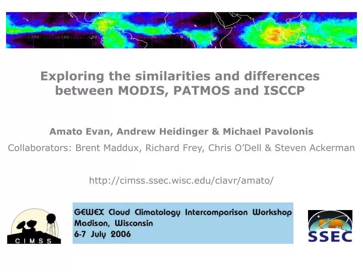
Exploring the similarities and differences between MODIS, PATMOS and ISCCP. Amato Evan, Andrew Heidinger & Michael Pavolonis Collaborators: Brent Maddux, Richard Frey, Chris O’Dell & Steven Ackerman http://cimss.ssec.wisc.edu/clavr/amato/. Outline. EOF analysis

E N D
Exploring the similarities and differences between MODIS, PATMOS and ISCCP Amato Evan, Andrew Heidinger & Michael Pavolonis Collaborators: Brent Maddux, Richard Frey, Chris O’Dell & Steven Ackerman http://cimss.ssec.wisc.edu/clavr/amato/
Outline • EOF analysis • PATMOS & ISCCP d2: total, high, mid & low cloud fractions • MODIS collection 5 total cloud fractions • NON-PHYSICAL time series comparisons • Discuss the effects of diurnal cycles • “Diurnally correct” time series • Conclusions • Significance of the findings • Future work
EOF Analysis • Remove the seasonality & ENSO then standardize every pixel • Reveal patterns in the data sets that may or may not be physical that explain the most variance • EOF maps are not rotated – variance in the EOF maps can be removed from the data set
EOF Analysis - PATMOS/AVHRR • Total Cloud Fraction - 1st EOF
EOF Analysis - PATMOS/AVHRR • Low & Mid Cloud Fraction - 1st EOF
EOF Analysis - PATMOS/AVHRR • High Cloud Fraction - 1st EOF
EOF Analysis - ISCCP • Total Cloud Fraction - 1st EOF
EOF Analysis - ISCCP • Low & Mid Cloud Fraction - 1st EOF
EOF Analysis - ISCCP • High Cloud Fraction
EOF Analysis - MODIS (2005 Terra: collection 5) • Total Cloud Fraction - 1st EOF
EOF Analysis - Summary • Each data set is probably influenced non-physical artifacts • may be driven by geometry or the algorithms • PATMOS & MODIS – artifacts may be more regional (poles) • PATMOS also has a ‘striping’ effect • ISCCP – Artifacts introduced by satellite geometry are pervasive
Time Series Analysis • Every data set contains measurements made at different times • AVHRR: changing sampling rates and over pass time (drift) • ISCCP: IR data is 3-hourly, VIS + IR is daytime only • MODIS: changing sampling rates • Since clouds have a diurnal cycle, maybe a comparison of the data sets should take observation times into account?
Time Series Analysis - Tropics Over Land • 15 S to 15 N • High Cloud Fractions • MODIS collection 4 daytime only!
Time Series Analysis - Tropics Over Land • High clouds • Not taking into account diurnal effects
Time Series Analysis - Tropics Over Land • High clouds • Strong diurnal cycle as seen by the satellites
Time Series Analysis - Tropics Over Land • Differences in satellite observation times
Time Series Analysis - Tropics Over Land • High clouds • Not taking into account diurnal effects
Time Series Analysis - Tropics Over Land • High clouds • Strong diurnal cycle as seen by the satellites
Time Series Analysis - Tropics Over Land • High clouds • Accounting for diurnal effects
Time Series Analysis - Tropics Over Land • High clouds • Accounting for diurnal effects
Time Series Analysis - Tropics Over Land • High cloud • Accounting for diurnal effects & standardizing
Not Corrected • Corrected Time Series Analysis - Tropics Over Water • High cloud
Comparison Time Series - Summary • Accounting for diurnal affects can greatly influence the results of a time series analysis (and probably a correlation analysis) • This effect is greatest in the presence of a strong diurnal cycle, generally over land • May be especially important when comparing two different polar orbiting satellites • These diurnal corrections for more regions and cloud types can be viewed at • http://cimss.ssec.wisc.edu/clavr/amato/
Exploring the similarities and differences between MODIS, PATMOS and ISCCP Conclusions • Each data set contains some artifacts that probably are not physical • However, when the diurnal cycle is considered, despite those artifacts, there is excellent agreement between all three data sets • Even when absolute cloud amounts are not in agreement, the data sets are still very well correlated
Exploring the similarities and differences between MODIS, PATMOS and ISCCP Future Work • Quantifying how the artifacts in the EOF analysis are affecting the long-term cloud signals • Possible to create a “best fit” cloud climatology that utilizes more that one data set • Similar to the work being done by Chris O’Dell • Use the diurnal information of ISCCP to “correct” the drift signal in the PATMOS data
Time Series Analysis - Tropics Over Land • Low clouds • Not taking into account diurnal effects
Time Series Analysis - Tropics Over Land • Low clouds • Strong diurnal cycle as seen by the satellites
Time Series Analysis - Tropics Over Land • Differences in satellite observation times
Time Series Analysis - Tropics Over Land • Effects of satellite drift
Time Series Analysis - Tropics Over Land • Low clouds • Not taking into account diurnal effects
Time Series Analysis - Tropics Over Land • Low clouds • Accounting for diurnal effects
Time Series Analysis - Tropics Over Land • Low clouds • Accounting for diurnal effects
Time Series Analysis - Tropics Over Land • Low clouds • Accounting for diurnal effects & standardizing
Time Series Analysis - Stratus Regions • Low clouds • Not taking into account diurnal effects
Time Series Analysis - Stratus Regions • Low clouds • diurnal cycle as seen by the satellites – approx. sine wave
Time Series Analysis - Stratus Regions • Low clouds • Not taking into account diurnal effects
Time Series Analysis - Stratus Regions • Low clouds • Accounting for diurnal effects
Time Series Analysis - Stratus Regions • Low cloud • Accounting for diurnal effects & standardizing
Time Series Analysis - Stratus Regions • Low clouds • Accounting for diurnal effects
Time Series Analysis - Stratus Regions • Low cloud • Accounting for diurnal effects & standardizing
EOF Analysis - Summary • Each data set is probably influenced non-physical artifacts • These artifacts may be driven by geometry or the algorithms • PATMOS & MODIS – artifacts may be more regional (poles) • PATMOS – Also has a ‘striping’ effect • ISCCP – Artifacts introduced by satellite geometry are pervasive
Exploring the similarities and differences between MODIS, PATMOS and ISCCP Conclusions • Each data set contains some artifacts that probably are not physical • When the diurnal cycle is considered, despite those artifacts, there is excellent agreement between all three data sets • Even when absolute cloud amounts are not in agreement, the data sets are still very well correlated
Exploring the similarities and differences between MODIS, PATMOS and ISCCP Future Work • Understand how the artifacts in the EOF analysis are affecting the long-term cloud signals • Possible to create a “best fit” cloud climatology that utilizes more that one data set • Similar to the work being done by Chris O’Dell