Download
1 / 15
150 likes | 523 Views
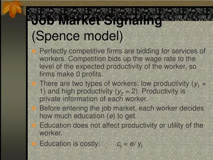
J ob M arket S ignaling (Spence model). Perfectly competitive firms are bidding for services of workers. Competition bids up the wage rate to the level of the expected productivity of the worker, so firms make 0 profits.

E N D
Job Market Signaling (Spence model) • Perfectly competitive firms are bidding for services of workers. Competition bids up the wage rate to the level of the expected productivity of the worker, so firms make 0 profits. • There are two types of workers: low productivity (y1 = 1) and high productivity (y2 = 2). Productivity is private information of each worker. • Before entering the job market, each worker decides how much education (e) to get. • Education does not affect productivity or utility of the worker. • Education is costly: ct = e/ yt
Job Market Signaling • After observing the level of e, firms make individual wage offers, which can depend on the level of education. • The goal of the firm is to maximize expected profit. • Workers maximize expected wage. • This game has many equilibria (pooling and separating) • The following is a separating PBE in this game: • Type 1 worker chooses e = 0, type 2 worker chooses e = 1; • Firms set wagesw(e<1) = 1, w(e>=1) = 2 • Firms believe that if e>=1 then type = 2 and if e<1 then type = 1
Limit pricing(Milgrom-Roberts model) • Limit pricing is a situation, where na incumbent monopolist charges a below-cost price to deter entry of a new firm (or „limit” the scale or scope of entry) • The classic rationale for limit pricing, that the entering firm will get scared of fierce competition, does not survivie the game-theoretic logic • Milgrom and Roberts (1982) showed that what looks like limit pricing could be an equilibrium in a signaling game
Limit pricing – the game • Nature decides the incumbent's type. His marginal cost is low with probability x or high with prob. (1 – x) • The incumbent sets the price, observed by the potential entrant. The entrant may update her beliefs about the incumbent based on that price • Entrant decides whether or not to enter. If no entry: incumbent enjoys unthreatened monopoly position. If entry occurs: firms receive duopoly profits
Limit pricing - notation • Let i=1 denote the incumbent and i=2 the entrant. • Mit(p) - monopoly profit of firm i if her type is t and charges price p • Mit = max Mit(p) - monopoly profit of firm i if her type is t and charges the price pmt(the optimal monopoly price for that type) • Dit - duopoly profit of firm i if incumbent's type is t • Assume that entrant wants to enter iff type is high, i.e. D2H > 0 > D2L(example: Bertrand competition with cH > cE > cL)
Separating equilibria • Let us look at conditions for and properties of separating equilibria in this game • In a separating equilibrium, the two types set different prices: pL pH • And entry will occur only if the entrant observes pH. It follows thatpH = pmH
Separating equil. cont. • We have the following constraints on pL: • ICH: M1H + D1H M1H(pL) + M1Hor M1H – M1H(pL) + (M1H – D1H)i.e. that the high-cost type will not rather mimic the low-cost type • IRL: M1L(pL) + M1L M1L + D1Lor M1L – M1L(pL) + (M1L – D1L)i.e. that the low-cost type would not rather deviate and charge pLm • In equilibrium, the entrant stays out if sees pL (satisfying the above), enters if sees any price other than pL (in particular pmH) (beliefs?)
Separating equil. cont. • It is not easy to prove that separating equilibria exist, but indeed they do, with pL < pLm(but not necessarily below cost) • the incumbent of type L has to give up some profit in order to discourage entry, the price is below monopoly price • social welfare is higher than under perfect information: entry occurs only when it is efficient and type L charges a below-monopoly price in period 1 (limit pricing of this type is good!)
Pooling equilibria • In a pooling equilibrium both types charge the same price pP • If (1 – x)D2H +xD2L > 0 then the entrant wants to enter if sees pP, but then at least one of the types has an incentive to charge a different price (i.e. Pooling equilibrium must involve entry deterrence) • We must therefore have (1 – x)D2H +xD2L < 0
Pooling equil. cont. • We have the following constraints on pP: • IRL: M1L(pP) + M1L M1L + D1Lor M1L – M1L(pP) + (M1L – D1L)i.e. that the low-cost type would not rather deviate and charge pLm • IRH: M1H(pP) + M1H M1H + D1Hor M1H – M1H(pP) + (M1H – D1H) i.e. that the low-cost type would not rather deviate and charge pHm • In equilibrium, the entrant stays out if sees pP (satisfying the above), enters if sees any price other than pP (beliefs?)
Pooling equil. cont. • It can be shown that there are many prices that satisfy the above conditions, but most importantly, pLmsatisfies them (intuitive) • The low-cost type does not have to worry about entry, so she chooses her monopoly price. The H type has to give up some profit to discourage entry, and charges pLm which is below her monopoly price • There is no entry in equilibrium no matter what the costs are (inefficient) • Social welfare effect is ambiguous: entry never occurs, but price sometimes lower
One more thing • Notice that in a separating equilibrium the L type is engaged in limit pricing, while in a pooling equilibrium - the H-type is engaged in limit pricing! • In both cases it is used as a deterrent by the type that is most endangered by entry.
Cooperative game theory • We do not model how the agents come to an agreement, we just characterize the players in terms of their bargaining power and then look for solutions that satisfy certain desirable mathematical conditions (axioms) • Axiomatic bargaining: the bargaining power is defined by the threat point • Coalitional Games: slightly more complex, bargaining power depends on threat points of every coalition. Coalition formation may be but does not have to be explicitly modeled or assumed.
Coalitional games • Coalitional game with transferable payoffs: the threat point of any coalition can be represented by a single number (the value of the coalition). We therefore assume that what a coalition can achieve can be turned into some transferable good (money?) and distributed among the coalition member in an arbitrary manner. The existence of the value of a coalition is assumed, the usual interpretation is that what coalition can achieve is independent of what happens outside of the coalition (if it isn’t, then non-cooperative GT is more appropriate). • Formally, the CG with transferable payoffs consists of: • N - the finite set of players • v(S) – the (value) function that assigns a real number to every nonempty set S N • Cohesiveness Assumption: v(N) ≥ the sum of values of any partition of N
The Core • The Core is the equivalent of NE for coalitional games • Let • The Core of a coalitional game is the set of payoff profiles x (N payoff vectors) for which x(S) ≥ v(S) for every S N • So x is in the core if no coalition can obtain a total payoff that exceeds the sum of its members’ payoffs in x • The core is a prediction of the level of transferable utility (money) that each player will end up with. Problem (just as with Nash equilibrium): may not be unique, may not exist.