Download
1 / 58
580 likes | 615 Views
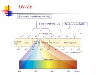
UCONN ECE 5212 092012016 (F. Jain) L4 1. Modulators using Optical transitions in quantum wells. 2.Photon absorption or emission involves electronic transitions

E N D
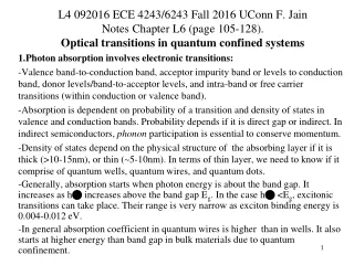
UCONN ECE 5212 092012016 (F. Jain)L4 1. Modulators using Optical transitions in quantum wells 2.Photon absorption or emission involves electronic transitions (Absorption is dependent on probability of transition and density of states; density of states depend on the physical structure of the absorbing layer if it is thick (>10-15nm), or thin). In terms of thin, we need to know if it comprise of quantum wells, multiple quantum wells, quantum wires, and quantum dots. Absorbing or emitting layer is made of direct gap or indirect gap semiconductors. Upward transitions involve photon absorption. These transitions are with and without phonons. In indirect semiconductors, phonon participation is essential to conserve momentum. Downward transitions result in photon emission. Transitions involve valence band-to-conduction band, band to impurity band or levels, donor-to-acceptor, and intra-band. Band-to-band transitions could involve free carriers or excitonic transitions.
Eg Ehh1 Fig. 1(a) E = 0 Optical Modulators using quantum confined Stark Effect We cover basics of exciton formation in quantum wells and related changes in the absorption coefficient and index of refraction. This phenomena is called confined Stark effect. Photon energy needed to create an exciton is given by h = Eg + (Ee1 + Ehh1) - Eex (Bulk Band gap) (Zero field energy of (Binding energy Electron and holes) of exciton) If the photon energy is greater than above equation, free electron and hole pair is created. Ee1
Electron wave function Hole wave function Fig. 1(b) Quantum well in the presence of E Application of perpendicular Electric Field When a perpendicular electric field is applied, the potential well tilts. Its slope is related to the electric field. • As E increases Ee & Eh decreases. As a result photon energy at which absorption peak occurs shifts to lower values (Red shift) . • The interaction between electron and hole wavefunctions (and thus, the value of the optical matrix elements and absorption coefficeint) also is reduced as magnitude E is increased. This is due to the fact that electron, hole wave functions are displaced with respect to each other. Therefore, the magnitude of absorption coefficient decreases with increasing electronic filed E.
MQW Modulator based on change in absorption due to quantum confined Stark effect Fig.3. Responsivity of a MQW diode (acting as a photodetector or optical modulator).
Phase Modulator: A light beam signal (pulse) undergoes a phase change as it transfers an electro-optic medium of length ‘L’ --------------- (1) In linear electro-optic medium …………………(2) E= Electric field of the RF driver; E=V/d, V=voltage and d thickness of the layer. r= linear electro-optic coefficient n= index
Figure compares linear and quadratic variation Dn as a funciton of field. MQWs have quadratic electro-refractive effect. Figure shows a Fabry-Perot Cavity which comprises of MQWs whose index can be tuned (Dn) as a funciton of field.
Mach-Zehnder Modulator Here an optical beam is split into two using a Y-junction or a 3dB coupler. The two equal beams having ½ Iin optical power. If one of the beam undergoes a phase change , and subsequently recombine. The output Io is related as Mach-Zehnder Modulator comprises of two waveguides which are fed by one common source at the input (left side). When the phase shift is 180, the out put is zero. Hence, the applied RF voltage across the waveguide modulates the input light.
Band to band transitions in nanostructures • Band to band free carrier transitions. • Band to band transitions involving exciton formation. • Light emission and absorption.
Energy bands Fig. 8 and 9. p.119
V(R) V0 2b<a -b 0 a a+b Energy bands (Ref. F. Wang, “Introduction to Solid State Electronics”, Elsevier, North-Holland) Fig. 13(b) and Fig. 13c. p.123-124
Absorption and emission of photons 1) (Transition Probability) here, (h) is the joint density of states in a volume V (the number of energy levels separated by an energy Fig. 2 p.138 2) Pmo probability that a transition has occurred from an initial state ‘0’ to a final state ‘m’ after a radiation of intensity I(h) is ON for the duration t. The joint density of states is expressed as Eq. 2B) o
Infinite Potential Well energy Levels Solve Schrodinger Equation In a region where V(x) = 0, using boundary condition that (x=0)=0, (x=L)=0. Plot the (x) in the 0-L region.
In the region x = 0 to x = L, V(x) = 0 Let (2) The solution depends on boundary conditions. Equation 2 can be written as D coskxx + C sinkxx. At x=0, (3) , so D= 0 nx = 1,2,3… (4) Using the boundary condition (x=L) = 0, we get from Eq. 3 sin kxL = 0, L = Lx
Page 52-53: Using periodic boundary condition (x+L) = (x), we get a different solution: We need to have kx= ---(6) The solution depends on boundary conditions. It satisfies boundary condition when Eq.6 is satisfied. If we write a three-dimensional potential well, the problem is not that much different ky = n y= 1,2,3,… kZ = , n z = 1,2,3,…. …(7) The allowed kx, ky, kz values form a grid. The cell size for each allowed state in k-space is …(8)
E N(E) VB k k+dk Density of States in 3D semiconductor film (pages 53, 54) Density of states between k and k+dk including spin N(k)dk = …(10) …11 Density of states between E and E+dE N(E)dE=2 E=Ec + (12) …(13) N(E)dE = …14 N(E)dE = …15
Energy Levels in a Finite Potential Well AlxGa1-xAs AlxGa1-xAs GaAs V(z) ∆EC ∆Ec = 0.6∆Eg ∆Ev = 0.4∆Eg 0 z 0 ∆Eg -EG z ∆EV -EG+∆EV
kL/2 αL/2 Where, radius is Output: Equation (15) and (12), give k, α’ (or α). Once k is known, using Equation (4) we get: The effective width, Leff can be found by: E1 is the first energy level. (4)
AlxGa1-xAs AlxGa1-xAs GaAs V(z) ∆EC ∆Ec = 0.6∆Eg ∆Ev = 0.4∆Eg 0 z 0 ∆Eg -EG z ∆EV -EG+∆EV Summary of Schrodinger Equation in finite quantum well region. (1) In the well region where V(x) = 0, and in the barrier region V(x) = Vo = ∆Ec in conduction band, and ∆Ev in the valence band. The boundary conditions are: (5) Continuity of the wavefunction (6) Continuity of the slope Eigenvalue equation:
C. 2D density of state (quantum wells) page 84 Carrier density number of states (1) Without f(E) we get density of states Quantization due to carrier confinement along the z-axis.
Photon Absorption Absorption coefficient a(hn) depends on type of transitions involving phonons (indirect) or not involving phonons (direct). Generally, absorption starts when photon energy is about the band gap. It increases as hv increases above the band gap Eg. It also depends on effective masses and density of states.(p.140, eqs 1-2) The absorption coefficient in quantum wires is higher than in wells. It also starts at higher energy than band gap in bulk materials. Absorption coefficient is related to rate of emission. Rate of emission in quantum wells is higher than in bulk layers. Rate of emission in quantum wires is higher than in quantum wells. Rate of emission in quantum dots is higher than in quantum wires. Rate of emission has two components: Spontaneous rate of emission Stimulated rate of emission.
·Direct and Indirect Energy Gap Semiconductors Semiconductors are direct energy gap or indirect gap. Metals do have not energy gaps. Insulators have above 4.0eV energy gap. Fig. 10b. Energy-wavevector (E-k) diagrams for indirect and direct semiconductors. Here, wavevector k represents momentum of the particle (electron in the conduction band and holes in the valence band). Actually momentum is = (h/2p)k = k
Effect of strain on band gap Ref: W. Huang, 1995 UConn doctoral thesis with F. Jain • Under the tensile strain, the light hole band is lifted above the heavy hole, resulting in a smaller band gap. • Under a compressive strain the light hole is pushed away from heavy. As a result the effective band gap as well as light and heavy hole m asses are a function of lattice strain. Generally, the strain is +/- 0.5-1.5%. "+" for tensile and "-" for compressive. • Strain does not change the nature of the band gap. That is, direct band gap materials remain direct gap and the indirect gap remain indirect.
Electrons & Holes Photons Phonons Statistics F-D & M-B Bose-Einstein Bose-Einstein Velocity vth ,vn 1/2 mvth2 =3/2 kT Light c or v = c/nr nr= index of refraction Sound vs = 2,865 meters/s in GaAs Effective Mass mn , mp (material dependent) No mass No mass Energy E-k diagram Eelec=25meV to 1.5eV ω-k diagram (E=hω) ω~1015 /s at E~1eV Ephotons = 1-3eV ω-k diagram (E= ω) ω~5x10¹³/s at E~30meV Ephonons = 20-200 meV Momentum P= k k=2π/λ λ=2πvelec/ω momentum: 1000 times smaller than phonons and electrons P= k k=2π/λ λ=2πvs/ω
(phonon absorption) + (phonon emission) p. 143 A= Direct and Indirect p.135 . Absorption coefficient a(hn) depends on type of transitions involving phonons (indirect) or not involving phonons (direct). Generally, absorption starts when photon energy is about the band gap. It increases as hn increases above the band gap Eg. It also depends on effective masses and density of states. (p.140, Eqs 1-2) The absorption coefficient in quantum wires is higher than in wells. It also starts at higher energy than band gap in bulk materials. Downward transitions result in photon emission. This is called radiative transition. When there is no photon emission it is called non-radiative transition. Rate of emission in quantum wells is higher than in bulk layers. Rate of emission in quantum wires is higher than in quantum wells. Rate of emission in quantum dots is higher than in quantum wires. Rate of emission has two components: Spontaneous rate of emission Stimulated rate of emission.
Quantum efficiency Absorption coefficient is related to rate of emission via Van Roosbroeck- Shockley. This enables obtaining an expression for radiative transition lifetime tr. There are ways to compute non-radiative lifetime tnr. The internal quantum efficiency is expressed as follows: Pr is the probability of a radiative transition. Two types of downward transitions. 1. Radiative transitions. 2. Non-radiative transition:
Absorption coefficient is related to rate of emission. Absorption coefficient is related to imaginary component of the complex index of refraction. Eq. 7 –page 214 is the rate of emission of photons at within an interval Van Roosbroeck - Shockley Relation under equilibrium Eq. 8 –page 214 Index of refraction nc is complex when there are losses. nc= nr – i k where extinction coefficient k = α/4pn, here alpha is the absorption coefficient. Also, nc is related to the dielectric constant. nc = = In non-equilibrium, we have excess electron-hole pairs. Their recombination gives emission of photons. The non-equilibrium rate of recombination Rc is In equilibrium,
Radiative life time in intrinsic and p-doped semiconductors (p.216) Nonradiative recombination: Auger Effect and other mechanisms (217) Nonradiative transitions are processes in which there are no photons emitted. Thus, there are several models by which energy is dissipated. Experimental observations are in terms of (1) emission efficiency, (2) carrier lifetime (coupled with emission kinetics), (3) behavior (or recombination mechanisms response) to temperature and carrier concentration variations. Recombination processes which are not associated with an emission of a photon are as follows: • Auger effect (carrier-carrier interaction) • Surface recombination, recombination through defects (Shah-Noyce-Shockley) • Multi phonon emission and others which may fit with the above proposed criterion. Since Auger processes involve carrier-carrier interactions, it is typical to assume that probability of occurrence of such a process should increase with the carrier concentrations.
e e First term: AnP Second Term: Bp2 h h Auger Transitions (p217-219) (n type semiconductor) (p type semiconductor)
E Density of states States in the Gap Density of states due to defects and inclusions Defect states caused nonradiative transitions Recombination via lattice defects or inclusions: Defects (dislocations, grain boundaries) and inclusions produce a continuum of energy states. These can trap electrons and holes which may recombine via continuum of states. Such a transition would be non-radiative. The energy states are distributed as: Nonradiative recombination: A microscopic defect or inclusion could induce a deformation of the band structure. e.g.
The absorption coefficient relations are in Chapter 3 Transitions involve: • Valence band-to-conduction band • Direct band-to-band • Indirect band-to-band • Band to band involving excitons (hn < Eg) • Band to impurity band or levels, • Donor level-to-acceptor level, and • Intra-band or free carrier absorption. Similar transitions in downward direction result in emission of photons.
Spectral width of emitted radiation Density of states in bulk is N(E)dE = The electron concentration ‘n’ in the entire conduction band is given by (EC is the band edge) This equation assumes that the bottom of the conduction band is =0. Electron and hole concentration as a function of energy
Graphical method to find carrier concentration in bulk or thick film (Chapter 2 ECE 4211)
Graphical method to find carrier concentration in quantum well
Spectral width in quantum well active layer is smaller than bulk thin film active layer Spectral width of emitted radiation
DEVICES based on optical transitionsEmission: LEDs Lasers PhotodetectorsAbsorption: Solar cellsOptical modulators and switchesOptical logic
Transitions in Quantum Wires: The probability of transition Pmo from an energy state "0" to an energy state in the conduction band "m" is given by an expression (derived in ECE 5212). This is related to the absorption coefficient a. It depends on the nature of the transition. The gain coefficient g depends on the absorption coefficient ain the following way: g = -a(1- fe - fh ). The gain coefficient g can be expressed in terms of absorption coefficient a, and Fermi-Dirac distribution functions fe and fh for electrons and holes, respectively. Here, fe is the probability of finding an electron at the upper level and fh is the probability of finding a hole at the lower level. Free carrier transitions: A typical expression for g in semiconducting quantum wires, involving free electrons and free holes, is given by:
Excitonic Transitions in Quantum Wires Excitonic Transitions: This gets modified when the exciton binding energy in a system is rather large as compared to phonon energies (~kT). In the case of excitonic transitions, the gain coefficient is: