Lab 6: Week 1 Quadrature Amplitude Modulation (QAM) Transmitter

1. Yeong Choo and Sam Kanawati Dept. of Electrical and Computer Engineering The University of Texas at Austin Lab 6: Week 1Quadrature Amplitude Modulation (QAM) Transmitter

2. Introduction • Digital Pulse Amplitude Modulation (PAM) Modulates digital information onto amplitude of pulse May be later upconverted (e.g. to radio frequency) • Digital Quadrature Amplitude Modulation (QAM) Two-dimensional extension of digital PAM Baseband signal requires sinusoidal amplitude modulation May be later upconverted (e.g. to radio frequency) • Digital QAM modulates digital information onto pulses that are modulated onto Amplitudes of a sine and a cosine, or equivalently Amplitude and phase of single sinusoid

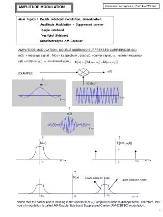
3. Review Y1(w) ½X1(w + wc) ½X1(w - wc) X1(w) ½ 1 w -wc - w1 -wc + w1 wc - w1 wc + w1 0 -wc wc w -w1 w1 0 Amplitude Modulation by Cosine • y1(t) = x1(t) cos(wct) Assume x1(t) is an ideal lowpass signal with bandwidth w1 Assume w1 << wc Y1(w) is real-valued if X1(w) is real-valued • Demodulation: modulation then lowpass filtering Baseband signal Upconverted signal

4. Review Y2(w) j ½X2(w + wc) -j ½X2(w - wc) X2(w) j ½ 1 wc wc – w2 wc + w2 w -wc – w2 -wc + w2 -wc w -j ½ -w2 w2 0 Amplitude Modulation by Sine • y2(t) = x2(t) sin(wct) Assume x2(t) is an ideal lowpass signal with bandwidth w2 Assume w2 << wc Y2(w) is imaginary-valued if X2(w) is real-valued • Demodulation: modulation then lowpass filtering Baseband signal Upconverted signal

5. Q d -d d I -d 4-level QAM Constellation Baseband Digital QAM Transmitter • Continuous-time filtering and upconversion Impulsemodulator gT(t) i[n] Index Pulse shapers(FIR filters) s(t) Bits Delay Serial/parallelconverter Map to 2-D constellation Local Oscillator + J 1 90o q[n] Impulsemodulator gT(t) Delay matches delay through 90o phase shifter Delay required but often omitted in diagrams

6. Baseband Digital QAM Transmitter Impulsemodulator gT(t) i[n] Index Pulse shapers(FIR filters) s(t) Bits Delay Serial/parallelconverter Map to 2-D constellation Local Oscillator + J 1 90o q[n] Impulsemodulator gT(t) 100% discrete timeuntil D/A converter i[n] L gT[m] s[m] cos(0m) Bits Index s(t) Serial/parallelconverter Map to 2-D constellation Pulse shapers(FIR filters) + sin(0 m) D/A J 1 L samples/symbol (upsampling factor) L gT[m] q[n]

7. 3 d d -d -3 d Q d -d d I -d 4-level QAM Constellation Average Power Analysis • Assume each symbol is equally likely • Assume energy in pulse shape is 1 • 4-PAM constellation Amplitudes are in set { -3d, -d, d, 3d } Total power 9 d2 + d2 + d2 + 9 d2 = 20 d2 Average power per symbol 5 d2 Peak Power per symbol 9 d2 • 4-QAM constellation points Points are in set { -d – jd, -d + jd, d + jd, d – jd } Total power 2d2 + 2d2 + 2d2 + 2d2 = 8d2 Average power per symbol 2d2 Peak power per symbol 2 d2 4-level PAM Constellation

8. The 16-Point Rectangular QAM Constellation

9. Q d -d d I -d 4-level QAM Constellation Performance Analysis of QAM • If we sample matched filter outputs at correct time instances, nTsym, without any ISI, received signal • Transmitted signal where i,k { -1, 0, 1, 2 } for 16-QAM • Noise For error probability analysis, assume noise terms independent and each term is Gaussian random variable ~ N(0; 2/Tsym)

10. 4-PAM vs 4-QAM Source: Appendix P in the Course Reader (EE445S)

11. 4-PAM vs 4-QAM Perspective 1: Take a vertical slice (at fixed SNR = 14dB) Source: Appendix P in the Course Reader (EE445S)

12. 4-PAM vs 4-QAM