Chapter 4 Properties of Regular Languages

Chapter 4 Properties of Regular Languages Pasbag, Turkey

Outline • 4.1 Proving Languages Not to Be Regular • 4.2 Closure Properties of Regular Languages • 4.3 Decision Properties of Regular Languages • 4.4 Equivalence and Minimization of Automata

4.1 Proving Languages Not to Be Regular • 4.1.1 Pumping Lemma for Regular Languages • Not every language is regular. • E.g., L01 = {0n1n | n 1} is not a regular language. • How to prove? Answer: use the pumping lemma. • In the sequel, we abbreviate “regular language” as “RL.”

4.1 Proving Languages Not to Be Regular • Theorem 4.1 Pumping lemma for RL’s Let L be an RL. Then, there exists an integer constant n (depending on L) such that for every string w in L with |w| n, we can break w into three substrings, w = xyz, such that: • ye (i.e., y has at least one symbol); • |xy| n; and • for all k 0, the “pumped” string xykz is also in L. Proof.See the textbook.

4.1 Proving Languages Not to Be Regular • (Supplemental) • The pumping lemma may be rewritten more precisely by mathematical notations as (L)(n)(w)(wL, |w| n  (x, y, z)(w = xyz, |xy| n, |y|  1, (k)(xykzL))).

4.1 Proving Languages Not to Be Regular • 4.1.2 Applications of Pumping Lemma • The pumping lemma may be used for proving “a given language isnot an RL,” instead of proving “is an RL.”

4.1 Proving Languages Not to Be Regular • 4.1.2 Applications of Pumping Lemma • Example 4.2 Prove the language Leq = {w | w has equal numbers of 0’s and 1’s} is not an RL.

4.1 Proving Languages Not to Be Regular • 4.1.2 Applications of Pumping Lemma Proof (by contradiction): • Assume that Leq is an RL. Then the pumping lemma says that there exists an integer n such that for every string w in L with length |w| n, w can be broken into 3 pieces, w = xyz, such that the three conditions 1~3 hold.

4.1 Proving Languages Not to Be Regular • In particular, pick the string w = 0n1n whose length is 2n. We know that w is in Leq. • Because|w| = 2n > n, by Theorem 4.1, string w can be broken into 3 pieces, w = xyz, so that • ye; • |xy| n; • for all k 0, xykzL.

4.1 Proving Languages Not to Be Regular • |xy| n says that xy consists of all 0’s because w = 0n1n . • Furthermore, yesaysy has at least one 0. (A) • Now, take k to be 0 and the pumping in the 3rd condition says that xy0z = xez = xz  L is true. (B)

4.1 Proving Languages Not to Be Regular • However, by (A) at least one 0 disappears when y was “pumped” out . • This means that the resulting string xz cannot have equal numbers of 0’s and 1’s, i.e., xz  L. Contradictive to (B) above! • So, the original assumption “Leq is an RL” is false (according to principle of “proof by contradiction.”). Done!

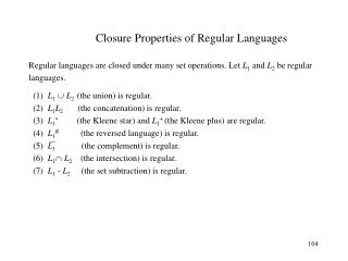
4.2 Closure Properties of RL’s • Closure means “being closed” in the same type of language domain, such as RL’s. • We will prove a set of “closure” theorems of the form --- “if certain languages are regular, and a language L is formed from them by certain operations, then L is also regular.”

4.2 Closure Properties of RL’s • Language operations for the above statement to be true include: • Union • Concatenation • Closure (star) • Intersection • Complementation • Difference • Reversal • Homomorphism • Inverse homomorphism

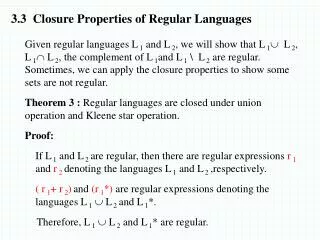
4.2 Closure Properties of RL’s • 4.2.1~4.2.4 (for proofs, see the textbook) • Let L and M be two RL’s over alphabet S. • Theorem 4.4 - the union L∪M is an RL. • Theorem 4.5 - the complement = S*L is an RL (S* is the universal language)

4.2 Closure Properties of RL’s • 4.2.1~4.2.4 (for proofs, see the textbook) • Theorem 4.8 - the intersection L∩M is an RL. • Theorem 4.10 - the difference LM is an RL. • Theorems – the concatenation LM and the closure L* are RL’s (no theorem numbers; mentioned in a frame on the top of p. 135).

4.2 Closure Properties of RL’s • The reversal of a string w = a1a2, … an is wR = anan-1…a2a1. • The reversalLR of a language L is the language consisting of the reversals of all its strings. • Theorem 4.11 --- the reversal LR of an RL L is also an RL.

4.2 Closure Properties of RL’s • A(string) homomorphismis a function h which substitutes a particular string for each symbol. That is, h(a) = x, where a is a symbol and x is a string. • Given w = a1a2…an, define h(w) = h(a1)h(a2)…h(an). • Given a language, define h(L) = {h(w) | wL}.

4.2 Closure Properties of RL’s • Example 4.13 • Let function h be defined as h(0)= ab and h(1) =e, then h is a string homomorphism. • For examples, 1. h(0011) = h(0)h(0)h(1)h(1) = ababee = abab. 2. If RE r = 10*1, then h(L(r)) = L((ab)*).

4.2 Closure Properties of RL’s • Theorem 4.14 - If L is an RL, then h(L) is also an RL where h is a homomorphism. • Inverse homomorphism: Let h be a homomorphism from some alphabet S to strings in another alphabet T. Let L be an RL over T. Then h1(L ) is the set of strings w such that h(w) is in L. • h1(L ) is read “h inverse of L.”

4.2 Closure Properties of RL’s • Example 4.15 --- • Let L = L((00 + 1)*) • Let (string) homomorphism h be defined as h(a) = 01, h(b) = 10. • It can be proved that h1(L) = L((ba)*) (see the textbook). • Theorem 4.16 - If h is a homomorphism from alphabet S to alphabet T, and L is an RL, then h1(L) is also an RL.

4.3 Decision Properties of RL’s • 4.3.1 Converting among Representations • Assume • #symbols = constant • #states = n. (for proofs, see the textbook) • Conversion from an e-NFA to a DFA --- requiring O(n32n) time in the worse cases • Conversion from a DFA to an NFA --- requiring O(n) time

4.3 Decision Properties of RL’s • 4.3.1 Converting among Representations • From an automaton (DFA) to an RE --- requiring O(n34n) time • From an RE to an automaton (e-NFA) --- requiring linear time in the size of the RE

4.3 Decision Properties of RL’s • 4.3.2 Testing Emptiness of RL’s • Testing if a regular language generated by an automaton is empty: • Equivalent to testing if there exists no path from the start state to an accepting state. • Requiring O(n2) time in the worse case. • Why? Time proportional to #arcs  each state has at most n arcs (to the n states)  at most n2 arcs  at most O(n2) time

4.3 Decision Properties of RL’s • 4.3.2 Testing Emptiness of RL’s • Testing if a language generated by an RE is empty: • A 2-step method: see the next page • A direct method: easy; see p. 154 of the textbook.

4.3 Decision Properties of RL’s • 4.3.2 Testing Emptiness of RL’s • A 2-step method for testing if a language generated by an RE is empty: • Convert the RE to an e-NFA --- requiring O(s) time as said previously, where s = |RE| (length of RE). • Test if the language of the e-NFA is empty --- requiring O(n2) time as said above. • The overall time requirement is O(s)+O(n2)

4.3 Decision Properties of RL’s • 4.3.2 Testing Emptiness of RL’s • Conclusion: The problem of testing emptiness of RL’s is decidable(i.e., there exists an algorithm to answer the problem). • Note: RL’s may be accepted by various automata (DFA’s, NFA’s, e-NFA’s) or generated by RE’s.

4.3 Decision Properties of RL’s • 4.3.3 Testing Membership in an RL • Membership Problem: given an RL L and a string w, is wL? • If L is represented by a DFA, the algorithm to answer the problem requires O(n) time, where n  |w| (# symbols in the string instead of #states of the automaton). • Why? Just processing input symbols one by one to see if an accepting state is reached.

4.3 Decision Properties of RL’s • 4.3.3 Testing Membership in an RL • If L is represented by an NFA without e-transitions, the algorithm requires O(ns2) time, where • n  |w| (# symbols in string winstead of #states) • s = #states • Why? Just processing input symbols one by one to see if an accepting state is reached, and at each state there are at most s2 choices of next states.

4.3 Decision Properties of RL’s • 4.3.3 Testing Membership in an RL • If L is represented by an e-NFA, the algorithm has to compute the e-closures at first before processing the symbols. • Computing e-closures requires O(s2)+O(s2)= O(s2) time (see the textbook). • Processing the input string of symbols needs nO(s2)=O(ns2) time. • Overall required time is O(ns2)

4.3 Decision Properties of RL’s • 4.3.3 Testing Membership in an RL • If L is represented by an REof size s, the algorithm first transforms it to an e-NFA with at most 2sstates in O(s) time, and then do as before (said in the last page). • Conclusion: The problem of testing the membership of an RL is decidable.

4.4 Equivalence & Minimization of Automata • What we want to show in this section: • Testing whether two descriptions of RL’s define the same languages. • Minimization of DFA’s --- • Good for implementations of DFA’s with less resources (like space, time, IC areas, …)

4.4 Equivalence & Minimization of Automata • 4.4.1 Testing Equivalence of States • Goal: want to understand when two distinct states p and q can be replaced by a single state that behaves like both p and q.

4.4 Equivalence & Minimization of Automata • 4.4.1 Testing Equivalence of States • Two states are said equivalent if for all strings w, (p, w) is an accepting state if and only if (q, w) is an accepting state. • Note: • It is not necessary to enter the same accepting state for the above definition to be met. • We only require that eitherboth states are acceptingorboth states are non-accepting.

4.4 Equivalence & Minimization of Automata • 4.4.1 Testing Equivalence of States • Non-equivalent states are said to be distinguishable. That is, state p is said to be distinguishable from q if there is at least a string w such that one of (p, w) and (q, w) is accepting, and the other is not accepting. • A systematic way to find distinguishable states --- use a table-filling algorithm (see the next page).

4.4 Equivalence & Minimization of Automata • 4.4.1 Testing Equivalence of States • Table-filling algorithm Basis. If p is an accepting state and q is not, then the pair {p, q} is distinguishable. Induction. • Let p and q be states such that for some input symbol a, the next states rd(p, a) and sd(q, a) are known to be distinguishable.Then {p, q} are distinguishable. (dist. pair r, s的前行者p, q也是dist. pair) • Why?See the next page. (dist. = distinguishable)

4.4 Equivalence & Minimization of Automata • 4.4.1 Testing Equivalence of States rd(p, a), sd(q, a) are distinguishable • There exists a string w such that only one of (r, w) and (s, w) is accepting. • But (p, aw) = (r, w), (q, aw) = (s, w) • There exists a string aw such that onlyone of (p, aw) and (q, aw) is accepting. • p and q are distinguishable.

4.4 Equivalence & Minimization of Automata • 4.4.1 Testing Equivalence of States • Example 4.19 --- apply the algorithm to the DFA shown in Fig. 4.18 (below).

4.4 Equivalence & Minimization of Automata • Basis: Since C is the only accepting state, we put an “x” into the pairs of {A, C}, {B, C}, {C, D}, {C, E}, {C, F}, {C, G}, {C, H}, with x meaning “distinguishable”.

4.4 Equivalence & Minimization of Automata • Induction: For the pair {C, H}, input 0 brings pair {E, F} to pair {C, H}, so {E, F} are distinguishable and the pair is marked.

4.4 Equivalence & Minimization of Automata • Find other pairs by using existing pairs (colored pairs are found from the bold red pair as “triggers” & subscripts are inputs). • Do this for all pairs in orderrecursively until no more pair can be marked.

4.4 Equivalence & Minimization of Automata • Final results are as follows. • The above method described in the textbook “wastes” some intermediate results. A better way is given next.

4.4 Equivalence & Minimization of Automata • A better way --- ( see 3rd paragraph, p. 160 in textbook)after finding distinguishable pairs by final states and mark them by “x” in the table, perform: • Set up a list for each pair in the table, initially empty. • For each unmarked pair {p, q}, do: • For each symbol a, compute rd(p, a), sd(q, a). • If any pair {r, s} is marked, then also mark the pair {p, q} as well as all the pairs in the list of the pair {p, q}, and also recursively all the pairs in the lists of just-marked pairs; elseput the pair {p, q} into the list of each pair of {r, s}. • Repeat the last step until no more pair in the table can be marked.

4.4 Equivalence & Minimization of Automata {r, s} = {B, G}, {F, C} with {F, C} already marked, so mark {p, q} = {A, B} {r, s} = {B, G}, {E, F} with both unmarked, so put {A, G} into lists of {B, G} and {E, F} {r, s} = {C, E} which is marked already, so mark {B, G} and also {A, G} in the list List = {A, G} List = {A, G}

4.4 Equivalence & Minimization of Automata • Final results are as follows. • Then, what???

4.4 Equivalence & Minimization of Automata • 4.4.1 Testing Equivalence of States • Theorem 4.20 If two states are not distinguishable by the table-filling algorithm, then they are equivalent. • 4.4.2 Taught later • 4.4.3 Minimization of DFA’s • Group equivalent states into a block and regard each block as a new state in the minimized DFA. • Take the block containing the old start state as the new start state. • Take the new accepting states as those blocks which contain old accepting states.

start Fig. 4.12 (identical to that in textbook except drawing style) 4.4 Equivalence & Minimization of Automata • 4.4.3 Minimization of DFA’s • Example 4.25 (cont’d from Example 4.19) • The final result below says (A, E), (B, H), (D, F) are equivalent states and can be put into 3 blocks as states of the new DFA. The final new DFA is as follows (right).

4.4 Equivalence & Minimization of Automata • 4.4.2 Testing Equivalence of RL’s • Use the table filling algorithm • Given two DFA’s AL and AM with start states qL and qM, respectively, for two RL’s L and M, we can test if their languages are equivalent by: • Imagine a third DFA A3 whose states are union of those of AL and AM. • Test if qL and qMare equivalent; if so, L and M areequivalent. • Why? Because accepting the same set of strings, i.e., the same set of languages. • See Example 4.21 for an example.

4.4 Equivalence & Minimization of Automata • 4.4.2 Testing Equivalence of RL’s • The table filling algorithm requires O(n2) time where n = #states. • Conclusion: The problem of testing the equivalence of two RL’s is decidable.

4.4 Equivalence & Minimization of Automata • 4.4.4 Why the Minimized DFA’s Can’t be Beaten • The minimized DFA by the table filling algorithm is really the “minimal,” having the fewest states in all DFA’s which accept the same language, as guaranteed by the following theorem. • Theorem 4.26If A is a DFA, and M the DFA constructed from A by the table filling algorithm, then M has as few states as any DFA equivalent to A.

Chapter 4 Properties of Regular Languages