Download
1 / 22
260 likes | 956 Views
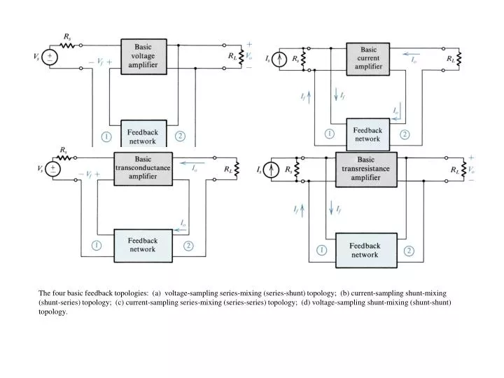
The four basic feedback topologies: (a) voltage-sampling series-mixing (series-shunt) topology; (b) current-sampling shunt-mixing (shunt-series) topology; (c) current-sampling series-mixing (series-series) topology; (d) voltage-sampling shunt-mixing (shunt-shunt) topology.

E N D
The four basic feedback topologies: (a) voltage-sampling series-mixing (series-shunt) topology; (b) current-sampling shunt-mixing (shunt-series) topology; (c) current-sampling series-mixing (series-series) topology; (d) voltage-sampling shunt-mixing (shunt-shunt) topology.
Fig. 8.8 The series-shunt feedback amplifier: (a) ideal structure; (b) equivalent circuit.
Fig. 8.9 Measuring the output resistance of the feedback amplifier of Fig. 8.8 (a): RofVt/I.
Fig. 8.10 Derivation of the A circuit and circuit for the series-shunt feedback amplifier. (a) Block diagram of a practical series-shunt feedback amplifier. (b) The circuit in (a) with the feedback network represented by its h parameters. (c) The circuit in (b) after neglecting h21.
Fig. 8.11 Summary of the rules for finding the A circuit and for the voltage-sampling series-mixing case of Fig. 8.10(a).
Fig. 8.13 The series-series feedback amplifier: (a) ideal structure; (b) equivalent circuit.
Fig. 8.14 Measuring the output resistance Rof of the series-series feedback amplifier.
Fig. 8.15 Derivation of the A circuit and circuit for the series-series feedback amplifiers. (a) A series-series feedback amplifier. (b) The circuit of (a) with the feedback network represented by its z parameters. (c) A redrawing of the circuit in (b) after neglecting z21.
Fig. 8.16 Finding the A circuit and for the current-sampling series-mixing (series-series) case.
Fig. 8.18 Ideal structure for the shunt-shunt feedback amplifier.
Fig. 8.19 Block diagram for a practical shunt-shunt feedback amplifier.
Fig. 8.20 Finding the A circuit and for the voltage-sampling shunt-mixing (shunt-shunt) case.
Fig. 8.22 Ideal structure for the shunt-series feedback amplifier.
Fig. 8.23 Block diagram for practical shunt-series feedback amplifier
Fig. 8.24 Finding the A circuit and for the current-sampling shunt-mixing (shunt-series) case.
Fig. 8.36 Bode plot for the loop gain A illustrating the definitions of the gain and phase margins.
Fig. 8.38 Frequency compensation for = 10-2. The response labeled A’ is obtained by introducing an additional pole at fD. The A” response is obtained by moving the original low-frequency pole to f’D.