Download
1 / 72
850 likes | 1.98k Views
Sampling Error. If probability methods are used, sampling is like drawing at random from a box, without replacement. The likely amount of chance (sampling) error in a simple random sample can be found if the population composition is known. Sampling Error.

E N D
Sampling Error • If probability methods are used, sampling is like drawing at random from a box, without replacement. • The likely amount of chance (sampling) error in a simple random sample can be found if the population composition is known.
Sampling Error • Example: A health study is based on a representative cross section of 6,672 Americans age 18 to 79. A sociologist wants to interview the participants, but only has resources to interview 100 people. There are 3,091 men in the study (46%) and 3,581 women (54%). If she uses simple random sampling, how far from the population proportion is her sample likely to be?
Sampling Error • The simple random sample is like drawing from a box without replacement. To count the number of men, use a 0-1 box model. 3,091 1 3,581 0
Sampling Error • If the sample size is small compared to the population size, the difference between drawing with or without replacement is insignificant. • Think of a chemist taking a single drop of solution from a large bucket.
Sampling Error • If the sample size is small compared to the population size, the difference between drawing with or without replacement is insignificant. • Think of a chemist taking a single drop of solution from a large bucket. • The expected number of men isThe expected percentage of men is 46%
Sampling Error • Key Concept: The sample percentage is likely different from the population percentage. But the expected value of the sample percentage equals the population percentage. EV for number = (sample size) x (population %) EV for percent = = population %
Sampling Error • The SD of the box is • So the SE is . The number of men is likely to be 46 give or take 5 or so. • The sample size is 100, so the percentage of men in the sample is likely to be 46% give or take 5% or so.
Sampling Error • The SE for a percentage is • We previously called this the “percent error.”
Sampling Error • The SE for a percentage is • We previously called this the “percent error.” • If we increase the sample size from 100 to 400, the expected percentage of men is still 46%, but the likely percent error is
Normal Approximation • According to the 2010 Census, the population of Winston-Salem age 18 and over is about 168,000. Of these, about 53.5% are female. As part of a pre-election survey, a simple random sample of 1500 people will be drawn from this population. Find the chance that the percentage of females in the sample is more than 56%.
Normal Approximation • Use a normal approximation. Find z-value using • Expected value for the percentage • SE for the percentage
Normal Approximation • Use a normal approximation. Find z-value using • Expected value for the percentage • SE for the percentage • EV for the percentage =
Normal Approximation • Use a normal approximation. Find z-value using • Expected value for the percentage • SE for the percentage • EV for the percentage = 53.5% • To find SE for the percentage, use a box model
Normal Approximation • Use a normal approximation. Find z-value using • Expected value for the percentage • SE for the percentage • EV for the percentage = 53.5% • To find SE for the percentage, use a box model 89,880 1 78,120 0
Normal Approximation • Use a normal approximation. Find z-value using • Expected value for the percentage • SE for the percentage • EV for the percentage = 53.5% • To find SE for the percentage, use a box model 89,880 1 78,120 0 • SD of box ≈ 0.5, SE for the percentage ≈ 1.3%
Normal Approximation • Find the z-value for 56%
Normal Approximation • Find the z-value for 56% • The probability that the percentage of females in the sample is more than 56% is less than 3% (about 2.87%).
Sampling Error • Increasing the sample size by a factor of N • Increases the SE for the number by a factor of . • Decreases the SE for the percentage by a factor of .
Sampling Error • Increasing the sample size by a factor of N • Increases the SE for the number by a factor of . • Decreases the SE for the percentage by a factor of . • KEY CONCEPT: If the sample is a small part of the population, the accuracy of the sample percentage is determined by absolute sample sizenotsample size relative to population size. • So bigger populations don’t need bigger samples to achieve the same accuracy.
How Large a Sample? • For simple random sampling,
How Large a Sample? • Suppose you want a sampling error of 1%. Then, • Example: 55% of people in Winston-Salem over age 25 attended college. The SD for a 0-1 box model for a simple random sample of this population is . To get a sampling error of 1%, the sample size should be .
Small Populations/Large Samples • There is a difference between drawing with and without replacement:
Small Populations/Large Samples • There is a difference between drawing with and without replacement: • When (# tickets) is much bigger than (# draws), and the SE’s are nearly equal. • Use CF when sample is >10% of population.
The BIG Question • If the population percentages are unknown, how accurate is the sample percentage likely to be?
The BIG Question • If the population percentages are unknown, how accurate is the sample percentage likely to be? • The problem: To compute SE, you need the SD of a 0-1 box model whose fraction of 1’s is unknown. • Moreover, the fractions of 1’s is often the number of interest.
The Bootstrap • The solution: Use the fractions of 1’s in the sample as an estimate of the fraction of 1’s in the box. • For large samples, this gives a good estimate of the SD. • Example: A simple random sample of 500 people age 18 to 24 is taken from a population of 100,000. Of the 500 sampled, 194 are currently enrolled in college.
The Bootstrap • of people in the sample attend college. • We take 38.8% as our estimate of the population percentage.
The Bootstrap • of people in the sample attend college. • We take 38.8% as our estimate of the population percentage. • A 0-1 box model for such a population has SD • Since 500 draws are made, the SE for the number of students in college is • The SE for the percentage is
Confidence Intervals • The sample percentage (38.8%) probably does not exactly equal the population percentage. • The SE for the percentage (2.18%) allows us to express our “confidence” in the estimate. 68% confidence interval: sample % 1(SE for %) 95% confidence interval: sample % 2(SE for %) 99.7% confidence interval: sample % 3(SE for %)
Confidence Intervals • We are about 68% confident that the population percentage is between 38.8% - 2.18% = 36.62% and 38.8% + 2.18% = 40.98%. • The 68% confidence interval for the population percentage is 36.62% to 40.98%. • The 95% confidence interval for the population percentage is 34.44% to 43.16%.
Confidence Intervals (handout: Confidence Intervals)
Interpretation • The 95% confidence interval does not mean that there is a 95% probability that the population percentage is between 36.44% and 43.16%. • That probability is either 0% or 100%. The variability is in the sampling not the parameter.
Interpretation • A different sample would give a different estimate of the population percentage and a different confidence interval. • The 95% refers to the likelihood that a confidence interval computed from a simple random sample contains the population percentage.
Visual Interpretation • Each time a population is sampled, a 95% confidence interval (vertical line) can be computed. In about 95% of the samples, the population percentage μ is in the interval.
Summary • Probabilities are useful for “forward reasoning” from a known box to a sample. • Confidence intervals are useful for “backward reasoning” from a known sample to an unknown box. • They make the following idea more precise: A sample percentage will be off the population percentage by an amount similar to the SE.
The Gallup Poll • Simple random sampling gives good results, but is impractical. How well do real polls do? • Example: Bush got 50.6% of the vote in 2004. With a simple random sample, SE for percent =
The Gallup Poll • Simple random sampling gives good results, but is impractical. How well do real polls do? • Example: Bush got 50.6% of the vote in 2004. With a simple random sample, SE for percent = .
Caution • When drawing with replacement from a 0-1 box, the number of 1’s follows the normal curve, as long as the number of draws is large. (Central Limit Theorem) • If the 0-1 box model is very lopsided, it takes a larger number of draws before the normal approximation takes hold. • Confidence intervals depend on the normal approximation, and maynot apply to a very lopsided box if the sample is fairly small.
Example (known population) • A box contains 1 red marble and 99 blues. 100 marbles are drawn at random with replacement. • EV for number of reds = 1 • SE for number of reds = 1 • Probability of drawing fewer than 0 reds = 0% • normal approximation estimates the probability is about 7%
Example (known population) • A box contains 1 red marble and 99 blues. 100 marbles are drawn at random with replacement. • EV for number of reds = 1 • SE for number of reds = 1 • Probability of drawing fewer than 0 reds = 0% • normal approximation estimates the probability is about 7% • The probability histogram for the number of 1’s in 100 draws does not follow the normal curve.
Example (unknown population) • Suppose a box contains 10,000 marbles, of which some are red and others are blue. To estimate the percentage of reds in the box, 100 marbles are drawn at random without replacement. Among the draws, 1 is red. • The percentage of reds in the box is estimated to be 1% with an SE of 1%. • Because the population seems to be lopsided, the normal approximation should not be used with a sample size of only 100. We do not assert that -1% to 3% is a 95% confidence interval.
Accuracy of Averages • The same machinery we used to predict sample percentages works just as well with averages. • When drawing at random from a box • EV for average of draws = average of box • SE for average of draws =
Predicting the Sample Average • A six-sided die will be rolled 100 times. • The average of the rolls will be about _____ give or take _____ or so.
Predicting the Sample Average • A six-sided die will be rolled 100 times. • The average of the rolls will be about 3.5 give or take .17 or so. • The chance that the average will be more than 3.7 is about
Predicting the Sample Average • A six-sided die will be rolled 100 times. • The average of the rolls will be about 3.5 give or take .17 or so. • The chance that the average will be more than 3.7 is about 11.5% ( z ≈ 1.2 )
Predicting the Average of the box • As before, • if the number of draws is small compared to the number of tickets, there is little difference between drawing with or without replacement • if the number of draws is large (in absolute terms) the SD of the sample is a good estimate for the SD of the box. • provided the box isn’t strongly skewed, confidence intervals for the average of the box can be found
Predicting the Average of the box • A simple random sample of 400 people age 25 and over is taken in a certain town in Appalachia. The average educational level of the sample is found to be about 11.6 years. The SD of the sample average is 4.1 years. • What is thebox model for this situation?
Predicting the Average of the box • Box model: one ticket for each person age 25 and over showing number of years of schooling completed by that person. 400 draws are made at random.
Predicting the Average of the box • Box model: one ticket for each person age 25 and over showing number of years of schooling completed by that person. 400 draws are made at random. • Bootstrap estimate: • avg. of box ≈ sample avg. = 11.6 years • SD of box ≈ SD of sample = 4.1 years