Download
1 / 28
280 likes | 350 Views
EPICS, exoplanet imaging with the E-ELT.

E N D
EPICS, exoplanet imaging with the E-ELT Markus Kasper, Jean-Luc Beuzit, Christophe Verinaud, Emmanuel Aller-Carpentier, Pierre Baudoz, Anthony Boccaletti, MariangelaBonavita, Kjetil Dohlen,Raffaele G. Gratton, Norbert Hubin, FlorianKerber, Visa Korkiaskoski, Patrice Martinez, Patrick Rabou, Ronald Roelfsema, Hans Martin Schmid, NiranjanThatte, Lars Venema, Natalia Yaitskova ESO, LAOG, LESIA, FIZEAU, OsservatorioAstronomicodiPadova, ASTRON, ETH Zürich, University of Oxford, LAM, NOVA 1
Outline Science goals (6s) Instrument and AO concept (12s) Science Output prediction (4s)
Exoplanets observations early 2009 Spectrum of HD 209458b Richardson et al., Nature 445, 2007 • ~ 300 Exoplanets detected, >80% by radial velocities, mostly gas giants, a dozen Neptunes and a handful of Super-Earths • Constraints on Mass function, orbit distribution, metallicity • Some spectral information from transiting planets HR 8799, Marois et al 2008 Beta Pic, Lagrange et al 2009 3
(Some) open issues • Planet formation (core accretion vs gravitational disk instability) • Planet evolution (accretion shock vs spherical contraction / “hot start”) • Orbit architecture (Where do planets form?, role of migration and scattering) • Abundance of low-mass and rocky planets • Giant planet atmospheres 4
Object Class 1, young & self-lumPlanet formation • in star forming regions or young associations • Requirements: • High spat. resolution of ~30 mas (3 AU at 100 pc, snow line for G-star) • Moderate contrast ~10-6 5
Object Class 2, within ~20 pcOrbit architecture, low-mass planet abundance ~500 stars from Paranal ± 30 deg, ~60-70% M-dwarfs • Requirements • High contrasts~10-9 at 250 mas (Jupiter at 20pc) • + spatial resolution ~10-8 at 40 mas (Gl 581d,~8 M) 6
Object Class 3, already known onesPlanet evolution and atmospheres discovered by RV, 8-m direct imaging (SPHERE, GPI) or astrometric methods (GAIA, PRIMA) From ESO/ESA WG report GAIA discovery space SPHERE discovery space 7
Concept 9
Concept: Achieve very high contrast Highest contrast observations require multiple correction stages to correct for Atmospheric turbulence Diffraction Pattern Quasi-static instrumental aberrations Diff. Pol. Visible diffraction suppression Coherence-based concept? XAO IFS Speckle Calibration,Differential Methods Diffraction + staticaberration correction XAO, S~90% Contrast ~ 10-3-10-4 Contrast ~ 10-9 Contrast ~ 10-6 NIR diffraction suppression x 1000 !
XAO concept Main parameters (baseline) Serial SCAOM4 / internal WFS, XAO XAO: roof PWS at 825 nm, 3 kHz 200x200 actuators (20 cm pupil spacing) AO + coro 1e-6 1e-7 RTC requirements:Efficient algorithms studied outside EPICS phase-A Numerical simulation, see poster of Visa Korkiakoski 11
High Order Testbench (HOT)Demonstrate XAO / high contrast concepts • Developed at ESO in collaboration with Arcetri and Durham Univ. • Turb. simulator, 32x32 DM, SHS, PWS, coronagraphy, NIR camera • H-band Strehl ratios ~90% in 0.5 seeing (SPIE 2008, Esposito et al. & Aller-Carpentier et al. ) correcting 8-m aperture for ~600 modes See poster of Aller-Carpentier
700K object next to K0 star HOT: XAO with APL coronagraph • Good agreement with SPHERE simulations • Additional gain by quasi-static speckle calibration (SDI, ADI)
HOT speckle stability 0 + 6hrs +30 hrs
Correction of quasi-static WFE incl. segments piston • DM “cleans” its control area from speckles • Need: measure static aberrations some nm level at science wavelength through residual turbulence (PD or Speckle Nulling) Standard WFE specs ok for most optics (near pupil) Concept to be demonstrated FP7 funded exp. (FFREE@LAOG and HOT)
HOT: Segments piston and correction of quasi-static WFE HOT pupil with DM and segmentation With segmentation
Residual PSF calibration Getting from systematic PSF residuals (10-6-10-7) to 10-8-10-9 Spectral Devonvolution (Sparks&Ford, Thatte et al.), Trade-off: spectral bandwidth vs inner working angle, IFS (baseline Y-H) Multi-band spectral or polarimetric differential imaging for smallest separation, needs planet “feature” (e.g. CH4 band, or polarization) IFS and differential polarimeter (600-900 nm) Coherence based methods (speckles interfere with Airy Pattern, a planet does not) Self-Coherent camera (see talk by P. Baudoz) Angular Differential Imaging (ADI) All
Speckle chromaticity and Fresnel SD needs “smooth” speckle spectrum -> near-pupil optics 20 nm rms at 10x Talbot 20 nm rms in pupil plane
Apodizer End-2-end analysis Apodizer only leads to improved final contrast APLC
E-ELT WFE requirements • Segment alignment (PTT) < 36 nm rms • Segment figuring < 50 nm rms • Segment high orders < 50 nm rms • M2-5, f>50 cycles/pupil < 30 nm rms • Roughness < 5 nm rms
Baseline Concept All optics near the pupil planeminimize amplitude errors and speckle irregular chromaticity
Predicted Science Output MC simulations • planet population with orbit and mass distribution from e.g. Mordasini (2007) • Model planet brightness (thermal, reflected, albedo, phase angle,…) • Match statistics with RV results Contrast model • Analytical AO model incl. realistic error budget • Spectral deconvolution • No diffraction or static WFE • Y-H, 10% throughput, 4h obs
Detection rates, nearby+young stars Mordasini et al. 2007 Contrast requirements
Summary • EPICS is the NIR E-ELT instrument for Exoplanet research • Phase-A to study concept, demonstrate feasibility by prototyping, provide feedback to E-ELT and come up with a development plan • Conclusion of Phase-A early 2010 • Exploits E-ELT capabilities (spatial resolution and collecting power) in order to greatly advance Exoplanet research (discovery and characterization)
END 28