Unsupervised Learning

1. STT592-002: Intro. to Statistical Learning Unsupervised Learning Chapter 10 Disclaimer: This PPT is modified based on IOM 530: Intro. to Statistical Learning

2. STT592-002: Intro. to Statistical Learning Outline • Principle Component Analysis (PCA) • What is Clustering? • K-Means Clustering • Hierarchical Clustering

3. STT592-002: Intro. to Statistical Learning Supervised vs. Unsupervised Learning • Supervised Learning: both X and Y are known • Unsupervised Learning: only X Supervised Learning Unsupervised Learning

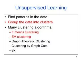
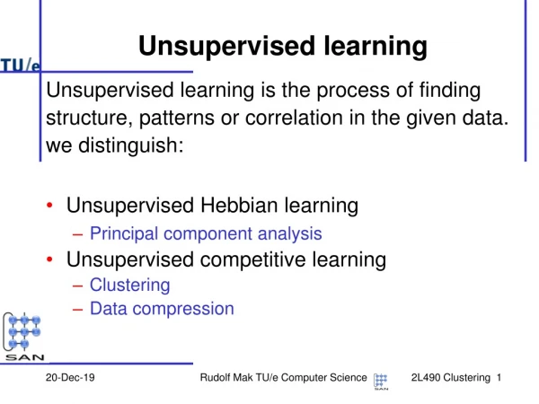
4. STT592-002: Intro. to Statistical Learning Overview of Unsupervised Learning • Focus on two particular types of unsupervised learning: • Principal Components Analysis (PCA), a tool used for data visualization or data pre-processing (dimension reduction) before supervised techniques are applied • Clustering: a broad class of methods for discovering • unknown subgroups in data.

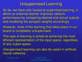
5. STT592-002: Intro. to Statistical Learning Challenge of Unsupervised Learning • Unsupervised learning is more challenging. • No simple goal for analysis, such as prediction of a response for classification or MSE. • More on exploratory data analysis. • Hard to assess the results from unsupervised learning, as we did not have any ground truth.

6. STT592-002: Intro. to Statistical Learning Examples of Unsupervised Learning • Eg: A cancer researcher might assay gene expression levels in 100 patients with breast cancer, and look for subgroups among the breast cancer samples, or among the genes, in order to obtain a better understanding of the disease. • Eg: Online shopping site: identify groups of shoppers with similar browsing and purchase histories, as well as itemsof interest within each group. Then an individual shopper can be preferentially shown the items likely to be interested, based on the purchase histories of similar shoppers. A search engine choose search results to display to a particular individual based on the click histories of other individuals with similar search patterns.

7. STT592-002: Intro. to Statistical Learning Principle Component Analysis (PCA) Review Chap 6.3, page 231-233

8. STT592-002: Intro. to Statistical Learning PCA • Ideas: a large set of correlated variables, principal components allow us to summarize this set with a smaller # of representative variables for original variability • Recall: PCA serves for -- • Dimension reduction: data pre-processing before supervised techniques are applied • Lossy data compression • Feature extraction • A tool for data visualization

9. STT592-002: Intro. to Statistical Learning PCA https://www.google.com/search?q=PCA&source=lnms&tbm=isch&sa=X&ved=0ahUKEwjx--iywp3UAhXESiYKHZGxAx0Q_AUICygC&biw=1229&bih=665 https://www.microsoft.com/en-us/research/people/cmbishop/?from=http%3A%2F%2Fresearch.microsoft.com%2F~cmbishop%2Fprml

10. STT592-002: Intro. to Statistical Learning PCA • Two common used definitions of PCA • Orthogonal Projection of the data onto a lower dimensional linear space, known as the principle subspace, such that the variance of the projected data is maximized; • Equivalently, as linear projection that minimizes average projection cost, where mean squared distance between data points and their projections. https://www.microsoft.com/en-us/research/people/cmbishop/?from=http%3A%2F%2Fresearch.microsoft.com%2F~cmbishop%2Fprml

11. STT592-002: Intro. to Statistical Learning USArrests Example Violent Crime Rates by US State This data set contains statistics, in arrests per 100,000 residents for assault, murder, and rape in each of the 50 US states in 1973. Also given is the percent of the population living in urban areas. A data frame with 50 observations on 4 variables. Murder: Murder arrests (per 100,000) Assault: Assault arrests (per 100,000) UrbanPop: Percent urban population Rape: Rape arrests (per 100,000) Q: Summarize a set of (X1, X2, X3, and X4) into a smaller # of representative variables for original variability.

12. STT592-002: Intro. to Statistical Learning PCA

13. STT592-002: Intro. to Statistical Learning PCA

14. STT592-002: Intro. to Statistical Learning PC loading and scores • PC loading vectors as the directions in feature space along which the data vary the most. • PC scores as projections along these directions.

15. Top/right: scale for loadings STT592-002: Intro. to Statistical Learning PCA calculation Standardize to mean 0 and SD=1 ## PC Scores for California: temp=c(0.2782682, 1.262814, 1.758923, 2.06782); pr.out_x1=sum(temp*c(0.5358995, 0.5831836, 0.2781909, 0.5434321)) pr.out_x1 ##2.498613 pr.out_x2=sum(temp*c(-0.4181809, -0.1879856, 0.8728062, 0.1673186)); pr.out_x2 ##1.5272427

16. STT592-002: Intro. to Statistical Learning PCA Biplot The figure represents both the principal component scores and the loadingvectors in a single biplot display. PCA loading: large positive scores on 1st component: California, Nevada and Florida, have high crime rates; While states like North Dakota, with negative scores on the first component, have low crime rates. California also has a high score on 2nd component, indicating a high level of urbanization, while the opposite is true for states like Mississippi. States close to zero on both components, such as Indiana, have approximately average levels of both crime and urbanization. 2nd Component: Level of Urbanization 1st Component: Serious Crime

17. STT592-002: Intro. to Statistical Learning PCA Biplot A biplot uses points to represent the scores of the observations on the principal components, and it uses vectors to represent the coefficients of the variables on the principal components. Interpreting Vectors: Vectors point away from origin in some direction. A vector points in directionwhich has the highest squared multiple correlation with the principal components. The length of the vector is proportional to the squared multiple correlation between the fitted values for the variable and the variable itself. 2nd Component: Level of Urbanization 1st Component: Serious Crime http://forrest.psych.unc.edu/research/vista-frames/help/lecturenotes/lecture13/biplot.html

18. STT592-002: Intro. to Statistical Learning More on PCA • Scaling of variables: • In general, we shall scale the data before performing PCA. • However, don’t scale the data if the variables may be measured in the same units (eg: gene data).

19. STT592-002: Intro. to Statistical Learning More on PCA • Uniqueness of the Principal Components: • Each principal component loading vector is unique, up to a sign flip. • But flipping the sign has no effect as the direction does not change. • The Proportion of Variance Explained (PVE):

20. STT592-002: Intro. to Statistical Learning More on PCA • Deciding How Many Principal Components to Use: • A n × p data matrix X has min(n − 1, p) distinct PCs. • Goal: choose smallest # of PCs to explain a sizable amount of the variation in the data. • Use the Scree Plot.

21. STT592-002: Intro. to Statistical Learning More on PCA • Scree Plot: Find the elbow in the scree plot. • Figure 10.4, one might conclude: a fair amount of variance is explained by first two PCs. There is an elbow after 2nd component. • After all, 3rd principal component explains less than 10% of the variance in the data, and the fourth principal component explains less than half that and so is essentially worthless.

22. STT592-002: Intro. to Statistical Learning Another Interpretation of Principal Components • Principal components provide low-dimensional linear surfaces that are closest to the observations.

23. STT592-002: Intro. to Statistical Learning Another Interpretation of Principal Components The first principal component loading vector has a very special property: it is the line in p-dimensional space that is closest to the n observations (using average squared Euclidean distance as a measure of closeness)

24. STT592-002: Intro. to Statistical Learning Another Interpretation of Principal Components The first two principal components of a data set span the plane that is closest to the n observations, in terms of average squared Euclidean distance.

25. STT592-002: Intro. to Statistical Learning Another Interpretation of Principal Components • Principal components provide low-dimensional linear surfaces that are closest to the observations.