Download

1 / 50
520 likes | 560 Views
TIME SERIES MODELS. Definitions. Forecast is a prediction of future events used for planning process . Time Series is the repeated observations of demand for a service or product in their order of occurrence. Quantity. Time. Components of a Time Series.

E N D
Definitions • Forecastis a prediction of future events used for planning process. • Time Seriesis the repeated observations of demand for a service or product in their order of occurrence.
Quantity Time Components of a Time Series • A time seriescan consist of five components. • Horizontal or Stationary – Fluctuations around a constant mean. • Long - term trend (T). • Cyclical effect (C). • Seasonal effect (S). • Random variation (R). A trend is a long term relatively smooth pattern or direction, that persists usually for more than one year.
6/97 12/97 6/98 12/98 6/99 A cycle is a wavelike pattern describing a long term behavior (for more than one year). Cycles are seldom regular, and often appear in combination with other components. 6/90 6/93 6/96 6/99 6/02 The seasonal component of the time series exhibits a short term (less than one year) calendar repetitive behavior.
Random variation comprises the irregular unpredictable changes in the time series. It tends to hide the other (more predictable) components. • Random or Irregular Variation –classifiedinto: • Episodic – unpredictable but identifiable • Residual – also called chance fluctuation and unidentifiable
Moving Average and Exponential Smoothing Methods • Consider models applicable to time series data with seasonal, trend, or both seasonal and trend component and stationary data. • Forecasting methods discussed can be classified as: • Averaging methods. • Equally weighted observations • Exponential Smoothing methods. • Unequal set of weights to past data, where the weights decay exponentially from the most recent to the most distant data points. • All methods in this group require that certain parameters to be defined. • These parameters (with values between 0 and 1) will determine the unequal weights to be applied to past data.
Moving Averages • A n-periodmoving average for time period t is the arithmetic average of the time series values for the n most recent time periods. • For example: A 3-period moving average at period (t+1) is calculated by (yt-2 + yt-1 + yt)/3
Centered Moving Average Method The centered moving average method consists of computing an average of n periods' data and associating it with the midpoint of the periods. For example, the average for periods 5, 6, and 7 is associated with period 6.
Moving Averages • A large k is desirable when there are wide, infrequent fluctuations in the series. • A small k is most desirable when there are sudden shifts in the level of series. • For quarterly data, a four-quarter moving average, MA(4), eliminates or averages out seasonal effects.
Moving Averages • For monthly data, a 12-month moving average, MA(12), eliminate or averages out seasonal effect. • Equal weights are assigned to each observation used in the average. • Each new data point is included in the average as it becomes available, and the oldest data point is discarded.
Summary of Moving Averages • Advantages of Moving Average Method • Easily understood • Easily computed • Provides stable forecasts • Disadvantages of Moving Average Method • Requires saving all past n data points • Lags behind a trend • Ignores complex relationships in data
Period Actual MA3 MA5 1 42 2 40 3 43 4 40 41.7 5 41 41.0 6 39 41.3 41.2 7 46 40.0 40.6 8 44 42.0 41.8 9 45 43.0 42 10 38 45.0 43 11 40 42.3 42.4 12 41.0 42.6 Simple Moving Average – Example (File: PPT_MA) • Consider the following data, • Starting from 4th period one can start forecasting by using MA3. Same is true for MA5 after the 6th period. • Actual versus predicted(forecasted) graphs are as follows;
Simple Moving Average - Example Actual MA5 MA3
Sample Excel analysis for Actual, Moving Averages for 3 and 5 periods
Sample Excel analysis for Actual, Centred Moving Averages for 2 and 4 periods
Sample SPSS analysis for Actual, Centered MA3 and Prior MA3 Period Actual MA3 Prior_MA3 1 42 2 40 41.7 3 43 41.0 4 40 41.3 41.7 5 41 40.0 41.0 6 39 42.0 41.3 7 46 43.0 40.0 8 44 45.0 42.0 9 45 42.3 43.0 10 38 41.0 45.0 11 40 42.3
Example: Weekly Department Store Sales • The weekly sales figures (in millions of dollars) presented in the following table are used by a major department store to determine the need for temporary sales personnel.
Example: Weekly Department Store Sales • Use a three-week moving average (k=3) for the department store sales to forecast for the week 24 and 26. The forecast for the week 26 is
Problem: Robert’s Drugs During the past ten weeks, sales of cases of Comfort brand headache medicine at Robert's Drugs have been as follows: Week Sales Week Sales 1 110 6 120 2 115 7 130 3 125 8 115 4 120 9 110 5 125 10 130 If Robert's uses a 3-period moving average to forecast sales, what is the forecast for Week 11?
Exponential Smoothing Methods • This method provides an exponentially weighted moving average of all previously observed values. • Appropriate for data with no predictable upward or downward trend. • The aim is to estimate the current level and use it as a forecast of future value.
Simple Exponential Smoothing Method • Formally, the exponential smoothing equation is • forecast for the next period. • = smoothing constant. • yt = observed value of series in period t. • = old forecast for period t. • The forecast Ft+1 is based on weighting the most recent observation yt with a weight and weighting the most recent forecast Ft with a weight of 1-
Simple Exponential Smoothing Method • The implication of exponential smoothing can be better seen if the previous equation is expanded by replacing Ft with its components as follows:
Simple Exponential Smoothing Method • If this substitution process is repeated by replacing Ft-1 by its components, Ft-2 by its components, and so on the result is: • Therefore, Ft+1 is the weighted moving average of all past observations.
Simple Exponential Smoothing Method • The exponential smoothing equation rewritten in the following form elucidate the role of weighting factor . • Exponential smoothing forecast is the old forecast plus an adjustment for the error that occurred in the last forecast.
Simple Exponential Smoothing Method • The value of smoothing constant must be between 0 and 1 • can not be equal to 0 or 1. • If stable predictions with smoothed random variation is desired then a small value of is desire. • If a rapid response to a real change in the pattern of observations is desired, a large value of is appropriate.
Measures of Forecast Errors • Cumulative Forecast Error (CFE) • Mean Squared Error (MSE) • Standard Deviation (σ) • Mean Absolute Deviation (MAD) • Mean Absolute Percent Error (MAPE)
Measures of Forecast Error Et = yt – Ft CFE = Et = MSE = MAD = MAPE = (Et – E)2 n– 1 Et2 n [|Et | (100)]/yt n |Et | n Choosing a MethodForecast Error
Example The following table shows the actual sales of upholstered chairs for a furniture manufacturer and the forecasts made for each of the last eight months. Calculate CFE, MSE, σ, MAD and MAPE for this product.
Absolute Error Absolute Percent Month, Demand, Forecast, Error, Squared, Error, Error, t ytFtEt Et2 |Et| (|Et|/yt)(100) 1 200 225 -25 625 25 12.5% 2 240 220 20 400 20 8.3 3 300 285 15 225 15 5.0 4 270 290 –20 400 20 7.4 5 230 250 –20 400 20 8.7 6 260 240 20 400 20 7.7 7 210 250 –40 1600 40 19.0 8 275 240 35 1225 35 12.7 Total –15 5275 195 81.3% Choosing a MethodForecast Error
Measures of Error Absolute Error Absolute Percent Month, Demand, Forecast, Error, Squared, Error, Error, tDtFtEt Et2 |Et| (|Et|/Dt)(100) 1 200 225 –25 625 25 12.5% 2 240 220 20 400 20 8.3 3 300 285 15 225 15 5.0 4 270 290 –20 400 20 7.4 5 230 250 –20 400 20 8.7 6 260 240 20 400 20 7.7 7 210 250 –40 1600 40 19.0 8 275 240 35 1225 35 12.7 Total –15 5275 195 81.3% CFE = – 15 – 15 8 E = = – 1.875 5275 8 MSE = = 659.4 195 8 s = 27.4 MAD = = 24.4 81.3% 8 MAPE = = 10.2% Choosing a MethodForecast Error
Measures of Forecast Accuracy • Choose MSE if it is important to avoid (even a few) large errors. Otherwise, use MAD / MAPE. • A useful procedure for model selection. • Use some of the observations to develop several competing forecasting models. • Run the models on the rest of the observations. • Calculate the accuracy of each model. • Select the model with the best accuracy measure.
Example: Robert’s Drugs During the past ten weeks, sales of cases of Comfort brand headache medicine at Robert's Drugs have been as follows: Week Sales Week Sales 1 110 6 120 2 115 7 130 3 125 8 115 4 120 9 110 5 125 10 130 If Robert's uses exponential smoothing to forecast sales, which value for the smoothing constant , = .1 or = .8, gives better forecasts?
Example: Robert’s Drugs • Exponential Smoothing To evaluate the two smoothing constants, determine how the forecasted values would compare with the actual historical values in each case. Let: Yt = actual sales in week t Ft = forecasted sales in week t F1 = Y1 = 110 For other weeks, Ft+1 = .1Yt + .9Ft
Example: Robert’s Drugs • Exponential Smoothing For = .1, 1 - = .9 F1 = 110 F2 = .1Y1 + .9F1 = .1(110) + .9(110) = 110 F3 = .1Y2 + .9F2 = .1(115) + .9(110) = 110.5 F4 = .1Y3 + .9F3 = .1(125) + .9(110.5) = 111.95 F5 = .1Y4 + .9F4 = .1(120) + .9(111.95) = 112.76 F6 = .1Y5 + .9F5 = .1(125) + .9(112.76) = 113.98 F7 = .1Y6 + .9F6 = .1(120) + .9(113.98) = 114.58 F8 = .1Y7 + .9F7 = .1(130) + .9(114.58) = 116.12 F9 = .1Y8 + .9F8 = .1(115) + .9(116.12) = 116.01 F10= .1Y9 + .9F9 = .1(110) + .9(116.01) = 115.41
Example: Robert’s Drugs • Exponential Smoothing For = .8, 1 - = .2 F1 = 110 F2 = .8(110) + .2(110) = 110 F3 = .8(115) + .2(110) = 114 F4 = .8(125) + .2(114) = 122.80 F5 = .8(120) + .2(122.80) = 120.56 F6 = .8(125) + .2(120.56) = 124.11 F7 = .8(120) + .2(124.11) = 120.82 F8 = .8(130) + .2(120.82) = 128.16 F9 = .8(115) + .2(128.16) = 117.63 F10= .8(110) + .2(117.63) = 111.53
Example: Robert’s Drugs • Mean Squared Error In order to determine which smoothing constant gives the better performance, calculate, for each, the mean squared error for the nine weeks of forecasts, weeks 2 through 10 by: [(Y2-F2)2 + (Y3-F3)2 + (Y4-F4)2 + . . . + (Y10-F10)2]/9
Example: Robert’s Drugs = .1 = .8 Week YtFt (Yt - Ft)2Ft (Yt - Ft)2 1 110 2 115 110.00 25.00 110.00 25.00 3 125 110.50 210.25 114.00 121.00 4 120 111.95 64.80 122.80 7.84 5 125 112.76 149.94 120.56 19.71 6 120 113.98 36.25 124.11 16.91 7 130 114.58 237.73 120.82 84.23 8 115 116.12 1.26 128.16 173.30 9 110 116.01 36.12 117.63 58.26 10 130 115.41 212.87 111.53 341.27 Sum 974.22 Sum 847.52 MSE Sum/9 Sum/9 108.25 94.17
Seasonal Analysis • Seasonal variation may occur within a year or within a shorter period (month, week) • To measure the seasonal effects we construct seasonal indices. • Seasonal indexes express the degree to which the seasons differ from the average time series value across all seasons.
For each time period compute the ratioyt/ytwhich removes most of the trend variation > This is based on the Multiplicative Model. > • For each season calculate the average of yt/ytwhich provides the measure of seasonality. • Adjust the average above so that the sum of averages of all seasons is 1 (if necessary) Computing Seasonal Indices • Remove the effects of the seasonal and random variations by regression analysis = b0 + b1t
Computing Seasonal Indices • Example • Calculate the quarterly seasonal indices for hotel occupancy rate in order to measure seasonal variation. • Data:
Computing Seasonal Indices • Perform regression analysis for the modely = b0 + b1t + e where t represents the time, and y represents the occupancy rate. Time (t) Rate 1 0.561 2 0.702 3 0.800 4 0.568 5 0.575 6 0.738 7 0.868 8 0.605 . . . . The regression line represents trend.
No trend is observed, but seasonality and randomness still exist. The Ratios > yt / yt • t yt Ratio • .561 .645 .561/.645=.870 • .702 .650 .702/.650=1.08 • …………………………………………………. =.639368+.005245(1)
The Average Ratios by Seasons • To remove most of the random variation • but leave the seasonal effects,average • the terms for each season. Average ratio for quarter 1: (.870 + .864 + .865 + .879 + .913)/5 = .878 Average ratio for quarter 2: (1.080+1.100+1.067+.993+1.138)/5 = 1.076 Average ratio for quarter 3: (1.221+1.284+1.046+1.122+1.181)/5 = 1.171 Average ratio for quarter 4: (.860 +.888 + .854 + .874 + .900)/ 5 = .875
(Seasonal averaged ratio) (number of seasons) Sum of averaged ratios Seasonal index = Adjusting the Average Ratios • In this example the sum of all the averaged ratios must be 4, such that the average ratio per season is equal to 1. • If the sum of all the ratios is not 4, we need to adjust them proportionately. Suppose the sum of ratios is equal to 4.1. Then each ratio will be multiplied by 4/4.1. In our problem the sum of all the averaged ratios is equal to 4: .878 + 1.076 + 1.171 + .875 = 4.0. No normalization is needed. These ratios become the seasonal indices.
17.1% above the annual average 117.1% 7.6% above the annual average 12.5% below the annual average 107.6% 87.8% 87.5% 12.2% below the annual average Quarter 1 Quarter 2 Quarter 3 Quarter 4 Quarter 1 Quarter 2 Quarter 3 Quarter 4 Interpreting the Seasonal Indices • The seasonal indexes tell us what is the ratio between the time series value at a certain season, and the overall seasonal average. • In our problem: Annual average occupancy (100%)
Actual series Smoothed series The linear trend (regression) line The Smoothed Time Series • The trend component and the seasonality component are recomposed using the multiplicative model. In period #1 ( quarter 1): In period #2 ( quarter 2):
Actual time series Seasonal index Seasonally adjusted time series = Deseasonalized Time Series By removing the seasonality, we can identify changes in the other components of the time series, that might have occurred over time.
There was a gradual increase in occupancy rate Deseasonalized Time Series In period #1 ( quarter 1): In period #4 ( quarter 2): In period #5 ( quarter 1):