Download
1 / 51
510 likes | 531 Views
5. Simplified Transport Equations.

E N D
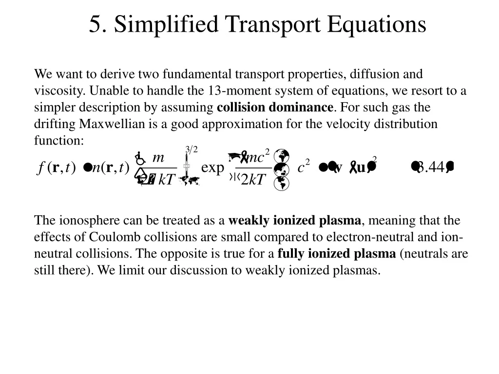
5. Simplified Transport Equations We want to derive two fundamental transport properties, diffusion and viscosity. Unable to handle the 13-moment system of equations, we resort to a simpler description by assuming collision dominance. For such gas the drifting Maxwellian is a good approximation for the velocity distribution function: The ionosphere can be treated as a weakly ionized plasma, meaning that the effects of Coulomb collisions are small compared to electron-neutral and ion-neutral collisions. The opposite is true for a fully ionized plasma (neutrals are still there). We limit our discussion to weakly ionized plasmas.
5.1 Basic Transport Properties (1) To develop the general idea, we assume an isothermal gas with a density n(x) that has a constant gradient in the -x direction, see Fig. 5.1a. We assume that the mean free path length , and that the velocity distribution is given by a non-drifting Maxwellian. We expect diffusion of particles from higher to lower density, i.e., from left to right in Fig. 5.1a. Let us calculate the net particle flux (# of particles per m2 and s) through the y-z plane at x. Appendix H.26 gives the thermal particle flux at x as [n(x) <c(x)>]/4 (HW#6: derive H.26). If the density n were constant, the net flux through the plane x = const would be zero because of the equal flux from the left and the right. The particles reaching the plane x had their last collision (in the average) in the plane x-x, where x ~ . The density at x-x is The particles arriving from the right had their last collision at x+x, and
5.1 Basic Transport Properties (2) The net particle flux crossing the plane at x then becomes
5.1 Basic Transport Properties (6)Example of Viscosity Effect (1) A gas flowing in the x direction between two infinite plates at y = 0 and y = a. Assume the plate at y = 0 is fixed and the plate at y = a moves in the x direction with velocity Vo. The particles close to y = a will tend to move with the plate in the x direction, while the particles at y = 0 will be at rest. What is the velocity at y? To find the answer we must solve the momentum equation (equation of motion, or force equation) (3.58):
5.1 Basic Transport Properties (7)Example of Viscosity Effect (2)
5.3 Transport in a weakly ionized plasma (1) Weakly ionized means that Coulomb collisions are of negligible importance in comparison with collisions with neutral particles. We start again with the momentum equation:
5.3 Transport in a weakly ionized plasma (2)Scale Analysis We start with the so-called diffusion approximation, for which the inertia terms can be neglected. To estimate the importance of the different terms look at the ratios.
5.3 Transport in a weakly ionized plasma (3) This means the first term in (5.23) can be neglected if Mj << 1, and t’, the time constant for the plasma processes, is long. Neglecting the time derivative eliminates the description of plasma waves. Summary: The diffusion approximation is valid for a slowly varying subsonic flow.
Consider a special case: no neutral wind (un = 0) and a dominant electric force due to an external field E0. 5.3 Transport in a weakly ionized plasma (4)
5.3 Transport in a weakly ionized plasma (5) To analyze the transport in a weakly ionized plasma (Coulomb collisions neglected) we start with the momentum and energy equations
5.11 Electric Currents and Conductivities (3) Since the electron mobility is much larger than the ion mobility, the current is carried by the electrons. The field-aligned current is therefore
6. Wave Phenomena6.1 General Wave Properties(1) Following Schunk’s notation, we use index 1 to indicate the electric and magnetic wave fields, E1 and B1, and the plasma variations, r1c, caused by the waves.The direction of the propagating wave is given by the propagation constant K. To find the plasma waves we must solve Maxwell’s differential equations in the plasma environment.
6.1 General Wave Properties(2) We solve Maxwell’s equations by taking the curl of (3):
6.2 Plasma Dynamics(1) The propagation of waves in a plasma is governed by Maxwell’s equations and the transport equations. We assume that the 5-moment simplified continuity, momentum, and energy equations (5.22a-c) can describe the plasma dynamics in the presence of waves. If we neglect gravity and collisions these equations become (Euler equations):
6.8 Electromagnetic Waves in a Plasma (1) Now we consider the case where E1 and B1are non-zero. We start with the general wave equation (6.20) assuming again a plane wave solution:
6.9 Ordinary and Extraordinary Waves (2) We can use the following equations:
6.11 Alfvén and Magnetosonic Waves Low frequency transverse (i.e. )electromagnetic waves are called: Alfvén waves, if magnetosonic waves, if The dispersion relations are, respectively:
9. Ionization and Energy Exchange Processes Solar extreme ultraviolet (EUV) is the major source of energy input into the thermospheres/ionospheres in the solar system. Electron precipitation contributes near the magnetic poles. l > 90 nm causes dissociation (O2O+O) l < 90 nm causes ionization Energy losses (sinks), from the ionosphere point of view, are airglow and the heating of the neutral atmosphere (thermosphere) Energy flow diagram in Fig. 9.1