Download
1 / 15
150 likes | 295 Views
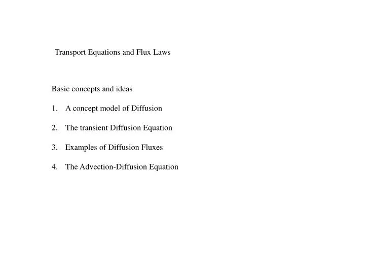
Transport Equations and Flux Laws. Basic concepts and ideas A concept model of Diffusion The transient Diffusion Equation Examples of Diffusion Fluxes The Advection-Diffusion Equation. A concept model for Diffusion. new. As an equation. Attribute of P at new time.

E N D
Transport Equations and Flux Laws • Basic concepts and ideas • A concept model of Diffusion • The transient Diffusion Equation • Examples of Diffusion Fluxes • The Advection-Diffusion Equation
A concept model for Diffusion new As an equation Attribute of P at new time We can use this equation to advance the evolution of the attributes at a point in time. Imagine “social” particles particles arranged and oscillating laterally on a lattice A given particle can only interact with its two nearest neighbors. the particle is determined to fit in and tries over time to take on the attributes of its neighbors –lets assume that there is a minimum time for the particle to achieve full social equilibrium. (based on the neighboring particle attributes at the beginning of the time step) old L P R
Particles in middle loose intensity Red Intensity particles at edge increase in intensity One example would be an initial top hat distribution (a set of red particles isolated in a sea of white particles) As we move from left to right in the domain How does the intensity of the red in the particles change
Time Approaches A steady state Another example is when the dye of the left most particle is continuously topped up to retain its intensity while the initial state of the other particles is white Fixed white Fixed red
old L P R new We can rewrite our equation as
Aside Assume (i) particles oscillate in a range +/- ½ of the lattice spacing (ii) that in a unit time the particle moves a unit distance with equal probability of going left of right (until it reaches its oscillation limit it which case its direction is reversed), and (iii) particles only have To meet once to come in “equilibrium” Simulation shows that when the particles are 2 units apart The expected meeting (equilibrium) time is 8 units 4 units apart The expected meeting (equilibrium) time is 32 units The expected meeting (equilibrium) time is 128 units 8 units apart So we can write Where a is a proportionality constant (m2/s) In this way
old L P R new We can rewrite our equation as Further in a more general setting we can check in on the progress of our solution at time steps Arriving at the update equation
L P R Captures interaction between particle at point P and particle at point R We can write this equation as
If the interactions occur faster on the left that the right we can adjust the value of the diffusivities L P R That is write Where If our particles were molecules we would expect very rapid times and short distances
The transient diffusion equation where Is the x component of flux (quantity/area/time) In an isotropic material
So we see that we will have a movement of quantity down a potential gradient In the model developed here we get the flow of quantity without macroscopic movement of the medium The molecules (particles) vibrate but the medium does not “flow” EXAMPLES In a general 3-D field The diffusive flux in an ISOTROPIC material is [quantity/area-time]
May which to write heat diffusive term as The advective flux x C = Cred C = 0 u Dx A fluid is moving down a pipe with velocity u. At time t the fluid to the left of a point x contains an immiscible (incapable of being mixed without separation of phases) dye at a concentration Cred. As the dye front moves through the box of length Dx its average concentration increases from C = 0 to C= Cred. What is the rate [moles/time] per unit area of dye entering the box qu = [moles/area-time] In general—the advective flux of a given quantity at a point in a flowing medium is a vector obtained by multiplying the velocity vector with the scalar [quantity/area-time] Diffusivity m2/s
n q Resolution of q in across Surface depends on surface orientation Total Flow across a surface element Consider a surface element of area dA and normal n in a flowing material which contains conserved scalar quantity n The Total flux at any point on the surface will be And the total quantity crossing the surface in the Opposite direction to the normal n is [quantity/ time]
Addendum n u Advective flux In opposite direction To normal -u.n Slope of f in direction of normal Diffusive flux in opposite direction To normal Direction of normal will control value of flux across surface. E.g. advection flux n n u n u u Zero Advec flux Max advec flux
n u(x,t) Conservation Balance—Steady State No Source Now consider a FIXED Arbitrary control volume located in A flowing material (velocity u) If there is no accumulation (steady state) or Generation or dissipation (Source/Sink) The net flow rate of a given quantity INTO the Volume has to be zero What goes in has to come out In math using the definition of the general flux By the divergence theorem But since volume V is chosen arbitrarily the argument in the integral must be identically zero At all points in the domain—leading to the general steady state diffusion-advection transport equation