Introduction to Bio-Inspired Models

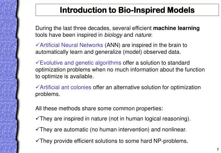
1. Introduction to Bio-Inspired Models • During the last three decades, several efficient machine learning tools have been inspired in biology and nature: • Artificial Neural Networks (ANN) are inspired in the brain to automatically learn and generalize (model) observed data. • Evolutive and genetic algorithms offer a solution to standard optimization problems when no much information about the function to optimize is available. • Artificial ant colonies offer an alternative solution for optimization problems. • All these methods share some common properties: • They are inspired in nature (not in human logical reasoning). • They are automatic (no human intervention) and nonlinear. • They provide efficient solutions to some hard NP-problems.

2. Introduction to Artificial Neural Networks Artificial Neural Networks are inspired in the structure and functioning of the brain, which is a collection of interconnected neurons (the simplest computing elements performing information processing): • Each neuron consists of a cell body, that contains a cell nucleus. • There are number of fibers, called dendrites, and a single long fiber called axon branching out from the cell body. • The axon connects one neuron to others (through the dendrites). • The connecting junction is called synapse.

3. Functioning of a “Neuron” • The synapses releases chemical transmitter substances. • The chemical substances enter the dendrite, raising or lowering the electrical potential of the cell body. • When the potential reaches a threshold, an electric pulse or action potential is sent down to the axon affecting other neurons.(Therefore, there is a nonlinear activation). • Excitatory and inhibitory synapses. weights (+ or -, excitatory or inhibitory) neuron potential: mixed input of neighboring neurons (threshold) nonlinear activation function

4. InputsOutputs Gradient descent Multilayer perceptron. Backpropagation algorithm 1. Init the neural weight with random values2. Select the input and output data and train it3. Compute the error associate with the output The neural activity (output) is given by a no linear function. 4. Compute the error associate with the hidden neurons 5. Compute and update the neural weight according to these values

5. Time Series Modeling and Forecast Sometimes the chaotic time series have a stochastic look difficult to predict An example is Henon map

6. xn+1 yn+1 zn+1 3:6:3 y y z 1 i i 3:k:3 W i k h h h 1 2 k 3:15:3 w k j x x x 2 3 j xn zn yn Example: Supervised Fitting and Prediction Given a time series with 2000 points (T=20), generated from a Lorenz system (chaotic behavior). To check modeling power different parameters are tested . Three variables (x,y,z) (xn,yn,zn) (xn+1,yn+1,zn+1) Continuous System Neural Network 3:k:3

7. Dynamical Behavior 3:6:3 A simple model doesn’t capture the complete structure of the system , then the dynamics of the system is not reproduce. A complex system it’s overfitting the problem and the dynamics of the system is not reproduce 3:15:3 Only a intermediate model with an appropriate amount of parameters can model the functional structure of the system and the dynamics

8. Xi Xi-1 Xi-2 Xi-3 Xi-j Time series from a infrared laser. Infrared laser intensity is modeled using a neural network. Only time lagged intensities are used. Net 6:5:5:1 The Neural network reproduces laser behavior The Neural Network can be synchronized with the time series obtained from the laser.

9. Structural Learning: Modular Neural Networks With the aim of giving some flexibility to the network topology, modular neural networks combine different neural blocks into a global topology. Fully-connected topology (too many parameters). Combining several blocks (parameter reduction). 2*4+4*4+4*1+9=37 weights Assigning different subnets to specific tasks we can simplify the complexity of the model. 2(2*2)+2(2*2)+4*1+9= 29 weights In most of the cases, block division is a heuristic task !!! How to obtain an optimal “block division” for a given problem ?

10. I x = F ( x , x ), x 3 1 2 F F y u F F z I x f + y - 1 f f u f z Functional Networks Functional networks are a generalization of neural networks which combine both qualitativedomain knowledge and data. Qualitative knowledge: Initial Topology Theorem. The simplest functional form is: Simplified Topology This is the optimal “block division” for this problem !!! Data: ( x , x , x ), i=1,2,... 1 i 2 i 3 i Learning (least squares): {f1, ..., fn} {a1, ..., an}

11. Some FN Architectures Separable Model: A simple topology. Associative Model: F(x,y) is an associative operator. Sliced-Conditioned Model: where f and y are covenient basis for the x- and y-constant slices.

12. A First Example. Functional vs Neural 100 points of Training Data with Uniform Noise in (-0.01,0.01). 25x25 points from the exact surface for Validation. Neural Network 2:2:2:1 MLP 15 parameters RMSE=0.0074 2:3:3:1 MLP 25 parameters RMSE=0.0031 Functional Network (separable model) F= {1,x ,x2 ,x3} 12 parameters RMSE=0.0024 Knowledge of the network structure (separable). Appropriate family of functions (polynomial). Non-parametric approach to learn the neuron functions !!!!

13. Functional Nets & Modular Neural Nets Advantages and shortcomings of Black-box topology with no problem connection. Neural Nets Efficient non-parametric models for approximating functions. Parametric learning techniques (supply basis functions). Functional Nets Model driven optimal topology. The topology of the network is obtained from the Functional network. The neuron functions are Approximated using MLPs. Hybrid functional-neural networks (Modular networks)

14. Another example. Nonlinear Time Series Nonlinear time series modeling is a difficult task because: Time series modeling and forecasting is an important problem with many practical applications. Sensitivity to initial conditions Trajectories starting at very close initial points split away after a few iterates. Goal: predicting the future using past values. x1, x2,…, xn ¿¿¿ xn+1 ??? X1=0.8 X1=0.8 + 10-3 Modeling methods: X1=0.8 - 10-3 xn+1 =F(x1, x2,…, xn) Fractal geometry There are many well-known techniques for linear time series (ARMA, etc.). Evolve in a irregular fractal space. Nonlinear time series may exhibit complex seemingly stochastic behavior. Nonlinear Maps (the Lozi model)

15. Separable Functional Net: ¿which basis family? F={sin(x),…,sin(mx), cos(x),…,cos(mx)} With 4*m parameters FN Symmetric Modular Functional Neural Net: 1:m:1 1:m:1 With 6*m parameters MFNN 1 Asymmetric Modular Functional Neural Net: 1:2m:1 1:2:1 With 2*m-2 parameters MFNN 2 Functional Models (separation) 500 training points 1000 validation points. m=11 (44 pars) RMSE=5.3e-3 m=7 (42 pars) RMSE=1.5e-3 m=7 (42 pars) RMSE=4.0e-4

16. Minimum Description Length Description Length for a model The Minimum Description Length (MDL) algorithm has proved to be simple and efficient in several problems about Model Selection.