Download
1 / 23
240 likes | 284 Views
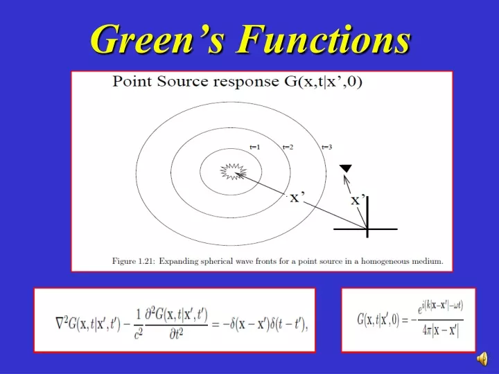
Green’s Functions. Outline. Attenuation Eikonal Eqn FD Solution to Eikonal Eqn Ray Tracing from T(x,z) Traveltime Integral Ray Tracing from ODE. If Q=1, then one wavelength traveled, amplitude diminishes by e^(-pi). Seismic Attenuation (Att. Mechanism=Fluid Sloshing).

E N D
Outline • Attenuation • Eikonal Eqn • FD Solution to Eikonal Eqn • Ray Tracing from T(x,z) • Traveltime Integral • Ray Tracing from ODE
If Q=1, then one wavelength traveled,amplitude diminishes by e^(-pi) Seismic Attenuation (Att. Mechanism=Fluid Sloshing) All these records differ from those associated with terrestrial earthquakes in lacking S (secondary or shear) waves. They also last for much longer than earthquakes - up to an hour, as though the Moon were "ringing" like a bell. The bulk of the moonquakes originate from depths of 600 km or more (attributed to the seismic signals bouncing back and forth in the low velocity surface layers [ejecta blanket]). They tend to occur in swarms associated both with preferred spatial locations and specific time intervals (probably accounted for by stresses induced by terrestrial tidal forces). Larger Q = smaller attenuation Smaller Q = greater attenuation Larger w = greater attenuation Smaller w = smaller attenuation Larger r = greater attenuation Note the two velocity discontinuities at about 20 and 60 km. Velocities within this interval are consistent with anorthosites. The higher velocities deeper than 60 km are associated with a proposed pyroxene-olivine upper mantle. Velocities between 4 and 20 km are indicative of a fractured basaltic flow sequence responding to load pressure. The shallow velocities (lower left inset) are attributed to the lunar ejecta blanket units discussed on the preceding page, overlain by comminuted regolith. If Q=1, then one wavelength traveled , amplitude diminishes by e^(-pi) If Q=2, then two wavelengths traveled , amplitude diminishes by e^(-pi) If Q=N, then N wavelengths traveled , amplitude diminishes by e^(-pi)
Outline • Attenuation • Eikonal Eqn • FD Solution to Eikonal Eqn • Ray Tracing from T(x,z) • Traveltime Integral • Ray Tracing from ODE
k + k = 1 2 2 x z w w c Plane wave (local homogeneous) 2 2 2 Apparent velocity T + T = 1 2 2 c 2 t(x,z)=2 z t(x,z)=1 x 2 2 2 (dt/dx) + (dt/dz) = (1/c) Eikonal Eqn. Eikonal Equation k + k = w 2 2 2 Dispersion Eqn. x z c 2 High freq. approx.
FD Soln of Eikonal Equation Step 1. Solve for times around src pt. by t=dr/c Times dr/c dr/c
dt/dx ~ FD Soln of Eikonal Equation 2 2 2 (dt/dx) + (dt/dz) = (1/c) 2 (Ta – Tb) 2 2 2 (Ta – Tb) + (Tc-Td) = s (Ta – Tb) s - 2 2 Td = Tc - 4dx 4dx 4dx 4dx 2 2 2 2dx d a b c Step 2. Solve for times around next grid by FD Pivot at p Replace PDE by FD: p b a dx
2 2 2 (Ta – Tb) + (Tc-Td) = s 2 2 2 (Ta – Tb) + (Tc-Td) = s 2 2 ( 2dx) ( 2dx) 2 2 2dx 2dx d b c FD Soln of Eikonal Equation Step 2. Solve for times around next grid by FD 2 2 2 (dt/dx) + (dt/dz) = (1/c) a dx
2 2 2 (Ta – Tb) + (Tc-Td) = s 2 2 ( 2dx) ( 2dx) FD Soln of Eikonal Equation Step 3. Solve for times around next grid by FD 2 2 2 (dt/dx) + (dt/dz) = (1/c)
FD Soln of Eikonal Equation Step 4. Repeat 2 2 2 (dt/dx) + (dt/dz) = (1/c) Apparent slowness
Problem: Calculation should expand along expand wavefronts Assume a heterogeneous v(x,y,z), such that the wavefrontT=10s is below Now find times associated with expanding square 10 s FD code makes mistake and finds 1st arrival time that is a horizontal ray
Eikonal FD Summary • Compute traveltime fields t(x,z) for each • Src. By a FD soln of Eikonal eqn. 2. t(x,z) used for traveltime tomography and migration. 3. First arrival energy not most energetic. Warning for migrationists. 4. First arrival energy for tomographers.
Outline • Attenuation • Eikonal Eqn • FD Solution to Eikonal Eqn • Ray Tracing from T(x,z) • Traveltime Integral • Ray Tracing from ODE
T(x+dx) dx along ray d = s ^ . dx = T ds ds Distance along ray T(x) x x+dx c T =1 Eikonal eqn. says Shooting Ray Tracing dx If we alreadt computed T then we are doing! But let’s assume no T computation and do shooting ray tracing. c (1) Desire to eliminate T dependency in eq. 1
T(x+dx) ( ) dx = T c ds d = s d = s ^ ^ . . dx = T dx = c T = T ds ds ds ds = c T ( ) T(x) dx ( ) ds d d 2 -2 = c ( ) T = c ( ) c = c - T ds ds c 2 2 2 Ray Tracing 1 c
dT Identity c T T ( ) ( ) ( ) ( ) T T |T| = = 2 2 [T] = [T] = ( ) | T| ( ) T T 2 2 ith component i k dT/dx[d/dx(dT/dx)] + +dT/dz[d/dz(dT/dx)] = 1/2d/dx[ (dT/dx)2 + (dT/dz)2] kth component dT/dx[d/dx(dT/dz)] + +dT/dz[d/dz(dT/dz)] = 1/2d/dz[(dT/dx)2 + (dT/dz)2]
T(x+dx) ( ) F(x) T(x) d d = = c c or 1st-order ODE’s - - ds ds dx c c 2 2 = F(x) c ds 0th-Order Shooting Ray Tracing ( ) dx c ds Specify start pt and direction 3 coupled 2nd-order ODE’s
T(x+dx) T(x) d = c - ds c 2 Crude Matlab Code for Homogeneous C (fx,fz) ( ) dx c ds Specify start pt and direction dx=lambda/10 x(1)=0;y(1)=0; % Initialize 2 endpoints for ray z(2)=dx;z(2)=dx % Initialize 2 endpoints for ray For i=1:nx x(3)=(2*x(2)-x(1))/2-c*fx(x(2),z(2)) ;%Solve above 2nd-order ODE for x(3) z(3)=(2*z(2)-z(1))/2-c*fz(x(2),z(2)) ;%Solve above 2nd-order ODE for z(3) x(1)=x(2);x(2)=x(3); % Reset 2 new endpoints for ray z(1)=z(2);z(2)=z(3); % Reset 2 new end points for ray end Start above loop again, except use two new starting endpoints of ray. Do this until a fan of rays have been traced from the same source point.
Beware Caustics: zero area, phase change x 0th-Order Shooting Ray Tracing Green’s Function 1. Shoot two neighboring rays from x’. 2. Measure area A(x|x’) at x x’ 3. G(x’|x) = W(t-T )/A(x|x’) A(x|x’)
dx = c T ds Interpolation Interpolation Shooting Ray Summary • Compute traveltime fields t(x,z) for each • Src. By a FD soln of Ray Equations. 2. t(x,z) used for traveltime tomography and migration. 3. Good for migration, avoid head waves. 3. Does not accurately handle caustics. Higher-order ray theory needed such as Maslov or Gaussian Beam.
Transmission Reflection A B x B * T = min(T + T ) * T = min(T ) AB Ax xB AB AB rays rays Fermat’s Principle • Stationary ray between two points is shortest traveltime ray = specular ray. (i.e., Snell’s law) A
Fermat’s Principle • Stationary ray between two points is shortest traveltime ray = specular ray. Multiple Reflection A B x’ x * T = ????????????????? AB