Download
1 / 88
880 likes | 889 Views
Network dimensioning and cost structure analysis + Introduction to HW3. Jan Markendahl November 30, 2015. Topics today. The network dimensioning part of the course How to estimate user demand Network dimensioning Cost structure analysis About HW3.

E N D
Network dimensioning and cost structure analysis+Introduction to HW3 Jan Markendahl November 30, 2015
Topics today • The network dimensioning part of the course • How to estimate user demand • Network dimensioning • Cost structure analysis • About HW3
About network dimensioning, deployment and cost structure analysis International spectrum allocation Regulating agencies Governments Standardization bodies EU EV A EV C EV D Bus A Bus C Bus E EV E EV B Bus B Bus D Bus E EV F Op A Op D Op C Op B ISP A ISP C ISP E ISP B ISP D ISP F
About network dimensioning, deployment and cost structure analysis • Economics of wireless infrastructure, scalability cost-capacity trade-offs, spectrum allocation • Network dimensioning, deployment and configuration strategies, impact of user demand • Cost structure modeling & analysis of network, to calculate CAPEX, OPEX, Net present value • Homework 3: Dimensioning and high level design of a wireless network incl. cost structure analysis
Homework 3 • For a specific user and traffic scenario you will • Make the dimensioning of a radio access network • Analyze the cost structure for different options GSM 900 UMTS 2100 GSM 1800 Transmission Buildout &Site costs Radio Equipment
The dimensioning problem Urban area Rural area HSPA UMTS GSM
The dimensioning problem • To satisfy the demand • To ”fill the demand box” with ”resource cylinders”
Agenda items • To estimate demand • Dimensioning of radio access network • Capacity, data rates and spectral efficiency of radio access technologies (RAT) • Trade offs using • Number of base station sites • Spectrum • Cell structure • What to do when the demand increases? • Cost structure analysis
Estimation of user demand • How to describe demand • Location of users • Number of users • Service mix • Traffic per user • How to estimate demand for dimensioning
Population density (persons per sqkm ) • Sweden average: 20 • Sweden rural araes: 1 – 10 • Sweden suburban areas: 100-1000 • Sweden urban areas: 1000 -10 000 • EU region rural areas: 100-200 • Malmö average: 2000 • Stockholm average: 4000 • Stockholm city: 25 000
Geografical data for Sweden Share of Inabitants Inh./km2 area population
Geografical data for Sweden Share of Inabitants Inh./km2 area population 92% of the population is living at 6 % of the total area 8% of the population is living at 95% of the total area
GSM coverageTele2 Telenor Telia ~70% covered area ~65% Covered area ~90% covered area
Estimation of user demand • The network dimensioning part of the course • How to describe demand • Location of users • Number of users • Service mix • Traffic per user • How to estimate demand for dimensioning
Traffic, prices and revenues Traffic and revenue for different services at the Swedish market Q4 2008 Estimated price per MByte for voice, SMS and data for one Swedish operator
Amounts of data – orders of magnitude (GB per month and person, 2010 Northern Europe) • Voice traffic 0,01-0,02 GB • Smartphones 0,10-0,20 GB • Laptop MBB as complement 1 – 5 GB • Laptop MBB as substitute 2 – 20GB • Fiber to the home (house hold) 100-200GB
Distribution of mobile broadband usage and subscriptions in Sweden Q4 2099 Share of subscriptions Share of data usage
Estimation of user demand • The network dimensioning part of the course • How to describe demand • Location of users • Number of users • Service mix • Traffic per user • How to estimate demand for dimensioning
Demand estimates as input for dimensioning of network capacity • Amount of data • per user, per time unit, per area unit • Usage: • Amount of data per user and time unit • Example 1: 100MB per day • Example 2: 5 GB per month • needs to be expressed as kbps-Mbps per user
Demand estimates as input for dimensioning of network capacity • Traffic • Amount of data per time unit per area unit • Depends on user density and usage per user • Example 1: 10 Mbps per sqkm • Example 2: 100 GB per day in a 2* 2 km area
Traffic density Urban area Suburban Rural area
Dimensioning Real time services • For voice and RT data you need to estimate the maximum number of ongoing calls or session • Is based on the traffic during the ”busiest hour”
Call Attempts 01:00 00:00 02:00 03:00 04:00 05:00 06:00 07:00 08:00 09:00 10:00 11:00 12:00 13:00 14:00 17:00 20:00 21:00 22:00 23:00 15:00 16:00 18:00 19:00 Time Capacity dimensioning – The busy hour
Call Attempts 01:00 00:00 02:00 03:00 04:00 05:00 06:00 07:00 08:00 09:00 10:00 11:00 12:00 13:00 14:00 17:00 20:00 21:00 22:00 23:00 15:00 16:00 18:00 19:00 Time Capacity dimensioning – The busy hour Blocked traffic Capacity that is deployed
Capacity dimensioning – Mobile broadband Montly demand of MBB spread out - all days of the month - all 24 hours of the day Time For NRT data traffic, the approach with”average data rate” per user can be used • X GB per user and month -> Y kbps per user
Capacity dimensioning – Mobile broadband Montly demand of MBB spread out - all days of the month - 12 out of 24 hours of the day Time
Capacity dimensioning – Mobile broadband Montly demand of MBB spread out - all days of the month - 8 out of 24 hours of the day Time
Short exercise • What is the average data rate per user? • Example A. • Monthlyusage 5.4 GB per user • Assume 30 days per month • Assume data usedduring 8 hours per day • Example B. • Monthlyusage 14.4 GB per user • Assume 20 (office) days per month • Assume data usedduring 4 hours per day • What is the average data consumption per month for thesecases? • Example C. • The operator promises at least 1 Mbps • Assuming data usage 1 hour per day • Example D. • The operator promises at least 8 Mbps • Assuming data usage 4 hours per day
Short exercise • What is the average data rate per user? • Example A. • Monthly usage 5.4 GB per user • Assume 30 days per month • Assume data used during 8 hours per day • Example B. • Monthly usage 14.4 GB per user • Assume 20 (office) days per month • Assume data used during 4 hours per day
Example of User demand – Mbps per sqkm Average data rate per user (Mbps)
Are these numbers realistic? • Population density • Stockholm average: 4000/ sqkm • Malmö average: 2000/ sqkm • Stockholm city: ~25 000/ sqkm • Penetration of mobile dongles • 20 % 2010 (may be 50% in the future) • Market share of operator ~ 40 % • Share of all users in an area: 0.2 * 0.4 = 8% • Check Mbps per sqkm!! - With 8% of all users • In area with 25 000 / sqkm => 2000 / sqkm • In area with 2 500 / sqkm => 200 / sqkm • In area with 250 / sqkm => 20 / sqkm
Homework 3 • For a specific user and traffic scenario you will • Make the dimensioning of a radio access network • Analyze the cost structure for different options GSM 900 UMTS 2100 GSM 1800 Transmission Buildout &Site costs Radio Equipment
Capacity of a base station? Bandwidth * spectralefficiency * No sectors/ spectrumreuse Bandwidth * No sectors/(spectrumreuse *spectralefficiency) Bandwidth * No sectors *spectrumreuse /spectralefficiency Bandwidth * No sectors * Spectralefficiency
Capacity of a base station – type? Bandwidth * No sectors * Spectral efficiency 5 MHz * 1 * 1 = 5 Mbps 10 MHz * 3 * 1 = 30 Mbps 20 MHz * 3 * 2 = 120 Mbps 20 MHz * 1 * 10 = 200 Mbps
Implications for network deployment • 1000 active users/sqkm, 50% market share=> deploy capacity for 500 users /sqkm • 5 GB usage per month per user~ 15 kbps per user 24 hours all days for one month~ 50 kbps per user during ”daytime” for one month • Capacity estimates for 500 users • 5 GB users: ~ 25 Mbps/sqkm • Compare with throughput for one ”cell” • ”3G” using 5 MHz ~ 3,5 Mbps • ”4G” using 20 MHz ~ 35 Mbps
Agenda items • To estimate demand • Dimensioning of radio access network • Capacity, data rates and spectral efficiency of radio access technologies (RAT) • Trade offs using • Number of base station sites • Spectrum • Cell structure • What to do when the demand increases? • Cost structure analysis
Traffic density • Estimate the demand • Number of users per area unit • Usage per user • Different types of users Urban area Suburban Rural area
Agenda items • To estimate demand • Dimensioning of radio access network • Capacity, data rates and spectral efficiency of radio access technologies (RAT) • Trade offs using • Number of base station sites • Spectrum • Cell structure • What to do when the demand increases? • Cost structure analysis
The dimensioning problem Urban area Rural area HSPA UMTS GSM
The dimensioning problem • To satisfy the demand • To ”fill the demand box” with ”resource cylinders”
Agenda items • To estimate demand • Dimensioning of radio access network • Capacity, data rates and spectral efficiency of radio access technologies (RAT) • Trade offs using • Number of base station sites • Spectrum • Cell structure • What to do when the demand increases? • Cost structure analysis
Bit rate and range – Bandwidth and Radio Access Technology (RAT) RAT 1 Macro BS
Bit rate and range – Bandwidth and Radio Access Technology (RAT) RAT 1 RAT 2 RAT 3 Macro BS
Bit rate and range – Bandwidth and Radio Access Technology (RAT) RAT 1 RAT 2 RAT 3 For a given amount of Spectrum ( e.g. X MHz) Macro BS
Bit rate and range – Bandwidth and Radio Access Technology (RAT) For twice the amount of Spectrum (2 X MHz) For a given amount of Spectrum ( e.g. X MHz) Macro BS