Making Predictions in an Uncertain World

1. Making Predictionsin an Uncertain World ?

2. Inductive Modeling Inductive Reasoning Fuzzy Inductive Reasoning Modeling the Error of a Prediction Economic Modeling Conclusions Table of Contents

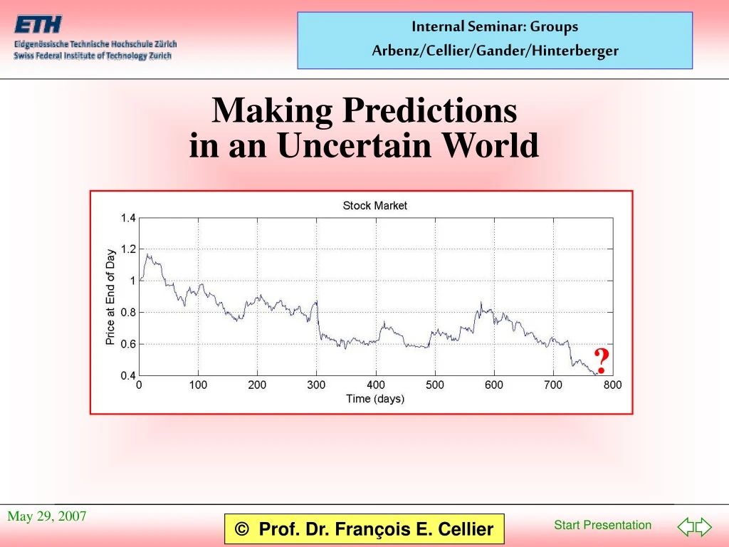
3. In this presentation, we shall study general techniques for identifying complex non-linear models from observations of input/output behavior. These techniques make an attempt at mimicking human capabilities of vicarious learning, i.e., of learning from observation. These techniques should be perfectly general, i.e., the algorithms ought to be capable of capturing an arbitrary functional relationship for the purpose of reproducing it faithfully. The techniques will also be totally unintelligent, i.e., their capabilities of generalizing patterns from observations are almost non-existent. Inductive Modeling

4. Knowledge-Based Approaches Observation-Based Approaches Deep Models Shallow Models SD Inductive Reasoners Neural Networks FIR Taxonomy of Modeling Methodologies

5. Observation-based modeling is very important, especially when dealing with unknown or only partially understood systems. Whenever we deal with new topics, we really have no choice, but to model them inductively, i.e., by using available observations. The less we know about a system, the more general a modeling technique we must embrace, in order to allow for all eventualities. If we know nothing, we must be prepared for anything. In order to model a totally unknown system, we must thus allow a model structure that can be arbitrarily complex. Observation-based Modeling and Complexity

6. ANNs are parametric models. The observed knowledge about the system under study is mapped on the (potentially very large) set of parameters of the ANN. Once the ANN has been trained, the original knowledge is no longer used. Instead, the learnt behavior of the ANN is used to make predictions. This can be dangerous. If the testing data, i.e. the input patterns during the use of the already trained ANN differ significantly from the training data set, the ANN is likely to predict garbage, but since the original knowledge is no longer in use, is unlikely to be aware of this problem. Parametric vs. Non-parametric Models

7. Non-parametric models, on the other hand, always refer back to the original training data, and therefore, can be made to reject testing data that are incompatible with the training data set. The Fuzzy Inductive Reasoning(FIR) engine that we shall discuss in this talk, is of the non-parametric type. During the training phase, FIR organizes the observed patterns, and places them in a data base. During the testing phase, FIR searches the data base for the five most similar training data patterns, the so-called five nearest neighbors, by comparing the new input pattern with those stored in the data base. FIR then predicts the new output as a weighted average of the outputs of the five nearest neighbors. Parametric vs. Non-parametric Models II

8. Training a model (be it parametric or non-parametric) means solving an optimization problem. In the parametric case, we have to solve a parameter identification problem. In the non-parametric case, we need to classify the training data, and store them in an optimal fashion in the data base. Training such a model can be excruciatingly slow. Hence it may make sense to devise techniques that will help to speed up the training process. Quantitative vs. Qualitative Models

9. How can the speed of the optimization be controlled? Somehow, the search space needs to be reduced. One way to accomplish this is to convert continuous variables to equivalent discrete variables prior to optimization. For example, if one of the variables to be looked at is the ambient temperature, we may consider to classify temperature values on a spectrum from very cold to extremely hot as one of the following discrete set: Quantitative vs. Qualitative Models II temperature = { freezing, cold, cool, moderate, warm, hot }

10. Given the system: 0 1 0 1 0 0 0 0 = 0 0 1 · x + 0 · u = 0 1 0 · x + 0 · u 1 0 -2 -3 -4 0 0 1 Inductive Reasoning: An Example · x = A · x + b · u y = C · x + d · u

11. Inductive Reasoning: An Example II • We simulate using a binary random input stream:

12. We recode (discretize) the three output signals by sorting each trajectory (array) separately and choosing the landmarks between different classes such that each class contains the same number of members. Let us recode each quantitative output trajectory into a qualitative output episode consisting of three classes. Hence we end up with a single binary input episode and three ternary output episodes. Our goal is to predict future values of the output episodes given future binary input values from observations of past input/output behavior. Recoding

13. Once the data have been recoded, we wish to determine, which among the possible sets of (past and current) variables best represent the observed (future) behavior. Of all possible combinations, we pick the one that gives us as deterministic an input/output relationship as possible, i.e., when the same input pattern is observed multiple times among the training data, we wish to obtain output patterns that are as consistent as possible. Each input pattern should be observed at least five times. Qualitative Modeling

14. Rule base y1(t) = f ( y3(t-2t), u2(t-t) , y1(t-t) , u1(t) ) Qualitative Modeling II

15. Qualitative Modeling III • The qualitative model is the optimal mask, i.e., the set of input patterns that best predict a given output. • Usually, the optimal mask is dynamic, i.e., the current output depends both on current and past values of inputs and outputs. • The optimal mask can then be applied to the training data to obtain a set of rules that can be alphanumerically sorted. • The rule base is our training data base.

16. Qualitative Simulation • We create one optimal mask for each output variable. • We can now shift the optimal masks beyond the measurement data, and predict the next output as the most likely output given the new input pattern. • We repeat this for each optimal mask and then continue to shift the masks further down using the already predicted data as “measurement” data. • In this way, we can predict future episodic behavior.

17. Qualitative Simulation II We got not a single prediction error.

18. Making Money Fast

19. Predicting Trajectory Behavior • Being able to predict episodic behavior is not sufficient for technical applications. We need to be able to predict trajectory behavior. • To this end, we require some kind of smoothing function that enables us to interpolate in between neighboring discrete class values. • Fuzzy logic can provide us with a good tool for this purpose.

20. Fuzzification proceeds as follows. A continuous variable is fuzzified, by decomposing it into a discrete class value and a fuzzy membership value. For the purpose of reasoning, only the class value is being considered. However, for the purpose of interpolation, the fuzzy membership value is also taken into account. Fuzzy variables are not discrete, but they are also referred to as qualitative. Fuzzy Variables

21. Systolic blood pressure = 141  { normal, 0.78 }  { too high, 0.18 } Systolic blood pressure = 110  { normal, 0.78 }  { too low, 0.15 } Fuzzy Variables II { Class, membership } pairs of lower likelihood must be considered as well, because otherwise, the mapping would not be unique.

22. Systolic blood pressure = 110 Systolic blood pressure = 141  { normal, 0.78, left }  { normal, 0.78, right } Fuzzy Variables in FIR FIR embraces a slightly different approach to solving the uniqueness problem. Rather than mapping into multiple fuzzy rules, FIR only maps into a single rule, that with the largest likelihood. However, to avoid the aforementioned ambiguity problem, FIR stores one more piece of information, the “side value.” It indicates, whether the data point is to the left or the right of the peak of the fuzzy membership value of the given class. right left

23. Discretization of quantitative information (Fuzzy Recoding) Reasoning about discrete categories (Qualitative Modeling) Inferring consequences about categories (Qualitative Simulation) Interpolation between neighboring categories using fuzzy logic (Fuzzy Regeneration) Fuzzy Inductive Reasoning (FIR)

24. FIR Crisp data Crisp data Fuzzy Recoding Regene- ration Fuzzy Modeling Fuzzy Simulation Fuzzy Inductive Reasoning (FIR) II

25. Fuzzification in FIR

26. Behavior Matrix Raw Data Matrix 2 Input Pattern Optimal Matrix 2 3 Matched Input Pattern 1 3 Euclidean Distance Computation dj 1 1 ? 5-Nearest Neighbors Output Computation fi=F(W*5-NN-out) Class Forecast Value Membership Side Qualitative Simulation in FIR

27. Time-series Prediction in FIR Water demand for the city of Barcelona, January 85 – July 86

28. Prediction Real Simulation Results

29. Deductive Modeling Techniques * have a large degree of validity in many different and even previously unknown applications * are often quite imprecise in their predictions due to inherent model inaccuracies Inductive Modeling Techniques * have a limited degree of validity and can only be applied to predicting behavior of systems that are essentially known * are often amazingly precise in their predictions if applied carefully Quantitative vs. Qualitative Modeling

30. Quantitative Subsystem Quantitative Subsystem FIR Model FIR Model Recode Recode Regenerate Regenerate Mixed Quantitative & Qualitative Modeling • It is possible to combine qualitative and quantitative modeling techniques.

31. Sources of Uncertainties in Predictions

32. Central Nervous System Control (Qualitative Model) Hemodynamical System (Quantitative Model) TH Heart Rate Controller Heart B2 Regenerate Regenerate Regenerate Regenerate Regenerate Myocardiac Contractility Controller Q4 Peripheric Resistance Controller Circulatory Flow Dynamics D2 Venous Tone Controller Carotid Sinus Blood Pressure Q6 Coronary Resistance Controller PAC Pressure of the arteries in the brain. Recode The Cardiovascular System

33. Simulation Results II

34. Discussion • The top graph shows the peripheric resistance controller, Q4, during a Valsalva maneuver. • The true data are superposed with the simulated data. The simulation results are generally very good. However, in the center part of the graph, the errors are a little larger. • Below are two graphs showing the estimate of the probability of correctness of the prediction made. It can be seen that FIR is aware that the simulation results in the center area are less likely to be of high quality.

35. Discussion II • This can be exploited. Multiple predictions can be made in parallel together with estimates of the likelihood of correctness of these predictions. • The predictions can then be kept that are accompanied by the highest confidence value. • This is shown on the next graph. Two different models (sub-optimal masks) are compared against each other. The second mask performs better, and also the confidence values associated with these predictions are higher.

36. Simulation Results III

37. We shall now deal with an application of Fuzzy Inductive Reasoning (FIR): making economic predictions. The presentation demonstrates how FIR can be used to improve the System Dynamics (SD) approach to soft-science modeling. It shows furthermore how hierarchical modeling can be used in the context of FIR, and demonstrates that by means of hierarchical modeling, the quality of economic predictions can dramatically be improved. Economic Modeling

38. One of the most daring (and dubious!) assumptions made by Forrester in his system dynamics approach to modeling soft-science systems was that a function of multiple variables can be written as a product of functions of a single variable each: This is obviously not generally true, and Forrester of course knew it. He made this assumption simply because he didn’t know how else to proceed. Birth_rate = Population · f1 (Pollution) · f2 (Food) · f3 (Crowding) · f4 ( Material_Standard_of_Living)  Birth_rate = Population · f (Pollution, Food, Crowding, Material_Standard_of_Living) Using FIR for Identifying Laundry Lists

39. An alternative might be to make use of FIR instead of table look-up functions for identifying any one of these unknown relationships among variables forming a laundry list. This is what we shall attempt now. Since FIR models are by themselves usually dynamic (since the optimal mask usually spans several rows), the functional relationships of each laundry list may furthermore be dynamic rather than static. Using FIR for Identifying Laundry Lists II

40. Modeling in the Agricultural Sector

41. In general, specific economic variables, such as food consumption patterns, depend on the general state of the economy. If the economy is doing well, Americans are more likely to consume steak, whereas otherwise, they may choose to buy hamburgers instead. The general state of the economy can in a first instance be viewed as depending primarily on two variables: availability of jobs, and availability of money. If people don’t have savings, they can’t buy much, and if they don’t have jobs, they are less likely to spend money, even if they have some savings. The general state of the economy is heavily influenced by population dynamics. It takes people to produce goods, and it takes customers to buy them. Modeling in the Agricultural Sector II

42. Demographic layer Three distinct layers are identified. Thespecific economic layerdepends on ageneric economic layer, which in turn depends on ademographic layer. Generic economic layer Each of therate variableshas a localdelay blockassociated with it. This delay block represents the fact that the rates are modeled usingFIR, which allows to obtaindynamic models of laundry lists. Specific economic layer Modeling in the Agricultural Sector III Food consumptionis modeled in ahierarchical fashion.

43. Contraceptives Food Supply The Great Depression Food Demand Macro-economy Population Dynamics Population Dynamics

44. One of the major difficulties with (and greatest strengths of) FIR modeling is its inability to extrapolate. Thus, if a variable is growing, such as the population, FIR has no means of predicting this directly. A simple trick solves this dilemma. Economists have known about this problem for a long time, since many other, mostly statistical, approaches to making predictions share FIR’s inability to extrapolate. When economists wish to make predictions about the value of a stock, x, they make use of the so-called daily return variable. Whereas x may be increasing or decreasing, the daily return is mostly stationary. x(end of day) – x(end of previous day) daily return = x(end of day) Prediction of Growth Functions

45.   IfP(t)is growing exponentially,k(t)is constant.  k(n+1) = FIR [ k(n), P(n), k(n-1), P(n-1), … ]  Prediction of Growth Functions II

46. 6 10 Predicting 1 year ahead. Predicting 3 years ahead. % Average error when predicting 1 year ahead. Food Supply Food Demand Average error when predicting 3 years ahead. Macro-economy Population Dynamics Population Dynamics II

47. $ % Average error incurred when making use of own past in predictions only Food Supply Food Demand Macro-economy Population Dynamics Average error found when making use of predicted population in economy predictions as well Macro-economy

48. % % Food Supply Food Demand Macro-economy Population Dynamics Macro-economy II The unemployment rate is a controlled variable. It is influenced by the lending rate. For many years, the feds tried to keep it around 6%. The variations around this value are difficult to predict accurately.

49. £ % Average error incurred when making use of own past in predictions only Food Supply Food Demand Macro-economy Population Dynamics Average error found when making use of population dynamics and economy forecasts as well Food Demand/Supply I

50. The models have shown that making use of predictions already made for the more generic layers of the architecture helps in improving the predictions of variables associated with the more specific layers. In most cases, the prediction errors are reduced by approximately a factor of three in this fashion. Notice that the best prediction techniques available were used in all cases. In particular, the confidence measure has been heavily exploited by always making several predictions in parallel, preserving in every step the one with the highest confidence value. Discussion III