Download
1 / 33
390 likes | 556 Views
Chemical Evolution of the Galaxy and its Satellites. Francesca Matteucci Cristina Chiappini Francesco Calura Antonio Pipino Gabriele Cescutti Universita’ di Trieste e OATS. How to model galactic chemical evolution. Initial conditions (open or closed-box; chemical composition of the gas)

E N D
Chemical Evolution of the Galaxy and its Satellites Francesca Matteucci Cristina Chiappini Francesco Calura Antonio Pipino Gabriele Cescutti Universita’ di Trieste e OATS
How to model galactic chemical evolution • Initial conditions (open or closed-box; chemical composition of the gas) • Birthrate function (SFRxIMF) • Stellar yields (how elements are produced and restored into the ISM) • Gas flows (infall, outflow, radial flow) • Equations containing all of of this...
The Stellar Birthrate • We define the stellar birthrate function as: • B(m,t) =SFRxIMF • The SFR is the star formation rate (how many solar masses go into stars per unit time) • The IMF is the initial stellar mass function describing the distribution of stars as a function of stellar mass
The parametrization of the SFR • The most common parametrization is the Schmidt (1959) law where the SFR is proportional to some power (k=2) of the gas density • Kennicutt (1998) suggested k=1.4 from studying star forming galaxies, but also a law depending on the rotation angular speed of gas and the first power of the gas density
The accretion history of the Galaxy • The gas infall rate can simply be constant in space and time • Or described by an exponential law:
Stellar Yields • Low and intermediate mass stars (0.8-8 Msun): produce He, N, C and heavy s-process elements. They die as C-O white dwarfs, when single, and can die as Type Ia SNe when binaries • Massive stars (M>8-10 Msun, core-collapse SNe): they produce mainly alpha-elements (O, Mg..), some Fe, light s-process elements and r-process elements and explode as core-collapse SNe • Type Ia SNe produce mainly Fe (0.6-0.7M_sun per SN)
Type Ia SN progenitors: SD model • Single-degenerate scenario (e.g. Whelan & Iben 1974; Han & Podsiadlowsky 2004): a binary system with a C-O white dwarf plus a MS star. When the star becomes RG it starts accreting mass onto the WD • When the WD reaches 1.44 Msun (Chandrasekhar mass), it explodes by C-deflagration as Type Ia supernova
Double-Degenerate scenario (Iben & Tutukov, 1984): two C-O WDs merge after loosing angular momentum due to gravitational wave radiation When the two WDs of 0.7 Msun merge, the Chandrasekhar mass is reached and C-deflagration occurs Type Ia SN progenitors: DD model
The clock for the explosion • Single-Degenerate model: the clock to the explosion is given by the lifetime of the secondary star, m2. The minimum time for the appearence of the first Type Ia SN is 30-35 Myr (the lifetime of a 8 Msun star) • Double-Degenerate model: the clock is given by the lifetime of the secondary plus the gravitational time-delay: 35 Myr + Delta_grav • Minimum delay time 1 Myr (Greggio 2005), maximum delay a Hubble time and more
The two-infall model of Chiappini, FM & Gratton (1997) predicts two main episodes of gas accretion During the first one the halo, bulge and part of thick disk formed, the second gave rise to the disk Exponential infall law with different timescales The two-infall model of Chiappini, FM & Gratton 1997
The predicted SFR The effect of a threshold gas density (7 Msun pc^(-2)) for the SF is evident The IMF is that of Scalo (1986) A gap in the SFR is predicted The star formation rate in the solar vicinity
[alpha/Fe] vs.[Fe/H] in the Solar Vicinity: Francois et al. 04
How do the gradients form? • If one assumes the disk to form inside-out, namely that first collapses the gas which forms the inner parts and then the gas which forms the outer parts • Namely, if one assumes a timescale for the formation of the disk increasing with galactocentric distance, the gradients are well reproduced if
Predicted and observed abundance gradients from Chiappini et al. (2001) Data from HII regions, PNe and B stars, red dot is the Sun The gradients slightly steepen with time (from blue to red) Predicted and Observed Abundance Gradients
The Galactic Bulge • Ballero, FM, Origlia & Rich (2007) proposed a model where the Bulge forms very quickly from gas shed by the halo • The star formation efficiency was quite high (starburst) and the IMF flatter than in the disk • In this situation a long plateau for [alpha/Fe] ratios is predicted
Do do the Dwarf Spheroidals form? • CDM models for galaxy formation predict dSph systems (10^7 Msun) to be the first to form stars (all stars should form < 1Gyr) • Then heating and gas loss due to reionization must have halted soon SF • Observationally, all dSph satellites of the MW contain old stars indistinguishable from those of Galactic globular clusters and they have experienced SF for long periods (>2 Gyr, Grebel & Gallagher, 04)
Modelling the dSphs • Lanfranchi & FM (03,04) computed the evolution of 6 dSphs: Carina, Sextan, Draco, Sculptor, Sagittarius and Ursa Minor • They assumed the SF histories as measured by the Color-Magnitude diagrams (Mateo, 1998;Dolphin 2002; Hernandez et al. 2000; Rizzi et al. 2003)
Model Lanfranchi & Matteucci (2004) SF history from Rizzi et al. 03. Four bursts of 2 Gyr, SF eff. = 0.15 Gyr^(-1) wind=7xSFR Salpeter IMF Results: Carina galaxy
Data from Koch et al. (2005) Best model from Lanfranchi & al. (2006) This model well reproduces also the [alpha/Fe] ratios in Carina The metallicity distribution of Carina
Model and data for Sculptor SF efficiency 0.05-0.5 Gyr^(-1), wind 7 XSFR One long SF episide lasting 7 Gyr Salpeter IMF Chemical evolution of Sculptor
Predicted and observed s- and r- process elements in Draco The effect of the time-delay between Type II and Ia SNe coupled with slow SF produces higher [s/Fe] than in the Milky Way Heavy elements in Sculptor
Blue line and blue data refer to Sculptor Red line and red data refer to the Milky Way The effect of the time-delay model is to shift towards left the model for Sculptor with a lower SF efficiency than in the MW Comparison Sculptor –Milky Way
Conclusions on the Milky Way • The Disk at the solar ring formed on a time scale not shorter than 7 Gyr • The whole Disk formed inside-out with timescales of the order of 2 Gyr in the inner regions and 10 Gyr in the outer regions • The inner halo formed on a timescale not longer than 2 Gyr • Time- delay model well explains abundance ratios. Nature of N still unknown (probably primary N from massive stars)
Conclusions on the Milky Way • The best model for the Bulge suggests that it formed by means of a strong starburst • The efficiency of SF was 20 times higher than in the rest of the Galaxy • The IMF was very flat, as it is suggested for starbursts • The timescale for the Bulge formation was 0.1 Gyr and not longer than 0.5 Gyr
Conclusions on dSphs • By comparing the [alpha/Fe] ratios in the MW and dSphs one concludes that they had different SF histories • The [alpha/Fe] ratios in dSphs are always lower than in the MW at the same [Fe/H], as a consequence of the time delay model and strong galactic wind
Conclusions on dSphs • Good agreement both for [s/Fe] and [r/Fe] ratios is obtained . These ratios are generally higher, for a given [Fe/H], than the corresponding ratios in S.N. • This is again a consequence of the time-delay model • It is unlikely that the dSphs are the building blocks of the MW