Download
1 / 35
350 likes | 575 Views
Raster Data Pixels as Modifiable Areal Units. E. Lynn Usery U.S. Geological Survey University of Georgia. Outline. MAUP Concepts from Socioeconomic Data Raster Resolution as MAUP Experimental Approach Results Conclusions. Objectives. Relate raster resolution effects to MAUP

E N D
Raster Data Pixels as Modifiable Areal Units E. Lynn Usery U.S. Geological Survey University of Georgia GIScience 2000
Outline • MAUP Concepts from Socioeconomic Data • Raster Resolution as MAUP • Experimental Approach • Results • Conclusions GIScience 2000
Objectives • Relate raster resolution effects to MAUP • Analyze effects of resolution on computation of parameters for water models • Develop empirical base for deciding appropriate resolution for particular modeling result • Examine pixels as modifiable units in database projection GIScience 2000
MAUP Concepts • Individuals in spatial analysis are often zones • Scientific study - definition of objects precedes measurement. • Not true for spatial data - areas are aggregated after data collected for one set of entities • Farm fields aggregated to counties for statistical analysis GIScience 2000
MAUP Concepts • No rules for aggregation; no standards; no international convention • Areal units for geographic study are arbitrary, modifiable, and subjective • Possible m zones from n individuals is combinatorial • 1000 objects (individuals) in 20 groups (zones) = 101260 • Does it matter? GIScience 2000
MAUP Scale Problem GIScience 2000
MAUP Scale Problem Male juvenile delinquency vs income based on 252 Census tracts (Gehlke and Biehl, 1934). Number of Units Correlation Coefficient 252 -0.5020 175 -0.5800 125 -0.6620 50 -0.6850 25 -0.7650 GIScience 2000
MAUP Aggregation Problem GIScience 2000
MAUP Aggregation Problem A.H. Robinson - grouping scheme correlations GIScience 2000
MAUP Solutions? • An insoluble problem; if so, ignore it • Problem that can be assumed away; work at individual level • Powerful analytical device; manipulate aggregations to get optimal zoning • Ruzycki (1994) - Used GIS to create 1000's of aggregations of census block groups in Milwaukee and calculated 3 indices of racial segregation for each aggregation; statistically analyzed results. GIScience 2000
Application of MAUP Concepts to Raster Data • Pixel is zone. • Various resolutions (pixel sizes) corresponds to scale problem of MAUP • Grouping of pixels in different ways to form larger units corresponds to the aggregation problem of MAUP GIScience 2000
Land Cover Example • Classify land cover from different image sources for same area using same classification system • Landsat TM (30 m) • SPOT MX (20 m) • Ikonos (4 m) • Do you get same percentages of land cover in each category? GIScience 2000
Water Modeling Example • Data collected at 30 m resolution • DEM • Land cover from TM • Aggregate data to get 10 acre (210 m) cells for parameter determination for AGNPS • How to aggregate? GIScience 2000
Experimental Approach • Analysis requires DEM, slope, and land cover at 30, 60, 120, 210, 240, 480, 960, 1920 m cells • Starting point is 30 m DEM and land cover • Calculate slope at 30 m cell size from DEM • Resample land cover • How to generate slope at 60 m and larger cell sizes? How to aggregate land cover? GIScience 2000
Method of Calculation • Slope calculated from DEM • 30, 60, 120, 210, 240, 480, 960, 1920 m cells • Compute slope from 30 DEM • Aggregate DEM from 30 m to each lower resolution • Compute slope from aggregated elevation data GIScience 2000
Sample of Slope Generation Approaches compute aggregate 30 m DEM 30 m slope 60 m slope aggregate compute 60 m slope 30 m DEM 60 m DEM aggregate compute 30 m DEM 120 m DEM 120 m slope 30 m DEM compute 30 m slope aggregate 120 m slope GIScience 2000
Results - DEM GIScience 2000
Results - DEM GIScience 2000
Image Results -- DEM 30-480 m Pixels 210-480 m Pixels GIScience 2000
Results -- Slope Slope % 30 to 480m Pixels 7.8816 7.8232 7.5870 7.8251 8.1604 8.5415 8.2065 7.9530 7.7434 7.7092 Slope % 210 to 480m Pixels 7.9514 7.8969 7.6244 7.7855 8.1263 8.5087 8.2157 7.8606 7.6390 7.6081 Regression Output: Constant 0.2762 Std Err of Y Est 1.1626 R Squared 0.7690 No. of Observations 500 Degrees of Freedom 498 X Coefficient(s) 0.8860 Std Err of Coef. 0.0218 GIScience 2000
Results -- Slope • Slope • Method of calculation affects results • Higher resolution aggregation directly to large pixel sizes yields better results than multistage aggregation (e.g., 30 m to 960 m is better than 30 m to 60 m to 120 m to 240 m to 480 m to 960 m) • Even multiples of pixels hold results while odd pixel sizes introduce error GIScience 2000
Slope Image Comparison 30 m to 480 m pixels 210 m to 480 m pixels GIScience 2000
Sample of Land Cover Aggregation Approaches aggregate aggregate 30 m LC 60 m LC 120 m LC aggregate aggregate 210m LC 30 m LC 120 m LC aggregate aggregate 30 m LC 210 m LC 480 m LC aggregate aggregate 30 m LC 960 m LC 1920 m LC GIScience 2000
Results - Land Cover -- 120 M Pixels GIScience 2000
Results - Land Cover -- 210 m Pixels GIScience 2000
Results - Land Cover -- 480 m Pixels GIScience 2000
Results-Land Cover -- 960 m Pixels GIScience 2000
Image Results - Land Cover 30-480 m Pixels 240-480 m Pixels GIScience 2000
Image Results - Land Cover 30-210 m Pixels 120-210 m Pixels GIScience 2000
Resampling Asia Land Cover • Land cover data (21 categories) at 1 km pixel size for Asia • Resample to 2,4,8,16,25, and 50 km pixels • Tabulate land cover percentages at each resolution to assess scale effects • Aggregate in various ways and retabulate to assess aggregation effects GIScience 2000
Asia Land Cover Lambert Azimuthal Equal Area Projection, 8 km pixels GIScience 2000
Scale Effect ResultsAsia Land Cover GIScience 2000
Aggregation Effect ResultsAsia Land Cover GIScience 2000
Conclusions • MAUP affects remotely sensed data • Resolution of images corresponds to MAUP scale problem • Resampling corresponds to MAUP aggregation problem • Higher resolution data are more accurate (scale effect) GIScience 2000
Conclusions • Areas of land cover vary significantly (up to 30 %) based on aggregation method • Nearest neighbor resampling leads to inaccurate aggregations based on modal category concepts • Continuous data (DEM and slope) retain values better through aggregation because of averaging (bilinear) during resampling. • Continental land cover datasets shows significant effects on land cover areas resulting from categorical (nearest neighbor) resampling. GIScience 2000