Download

1 / 37
380 likes | 543 Views
DMAIC: Improve. Robert Setaputra. Objective. Ready to develop, test, and implement solutions to improve the process by reducing variation in the critical output variables caused by the vital few of input variables. Small note.

E N D
DMAIC: Improve Robert Setaputra
Objective • Ready to develop, test, and implement solutions to improve the process by reducing variation in the critical output variables caused by the vital few of input variables.
Small note • In many cases, it is difficult to completely separate the activities in Measure, Analyze, and Improve.
Design of Experiment (DOE) • DOE is a collection of statistical methods for studying the relationships between independent variables, and their interactions (also called factors, input variables, or process variables) on a dependent variable (or CTQ).
Design of Experiment (DOE) 23.5 24.6 Factors Replications Levels
Design of Experiment (DOE) • Full factorial • All possible combinations • No prior knowledge about the subject • 2k = k factors each with 2 levels • 22 = 2 factors each with 2 levels • Fractional factorial • Excluding some combinations • Preferred when it is costly to do experiments • 2k-1 = k-1 factors each with 2 levels
Design of Experiment (DOE) • ANOVA One Factor • ANOVA Two Factor Remember Gage R&R with ANOVA?
Correlation Coefficient • The sample correlation coefficient (r) measures the degree of linearity in the relationship between X and Y • -1 <r< +1
Notes on Correlation Coefficient • Correlation is a measure of linear association and not necessarily causation • Just because two variables are highly correlated, it does not mean that one variable is the cause of the other, and vice versa.
Notes on Correlation Coefficients How about this one? Do you think there is no correlations between X and Y? Remember that rxy only measures linear correlation. Obviously, the above shows no correlations between X and Y
Example • A golfer is interested in investigating the relationship, if any, between driving distance and 18-hole score Average Driving Distance (yds.) Average 18-Hole Score 69 71 70 70 71 69 277.6 259.5 269.1 267.0 255.6 272.9
Example (cont’d) x y 69 71 70 70 71 69 -1.0 1.0 0 0 1.0 -1.0 277.6 259.5 269.1 267.0 255.6 272.9 10.65 -7.45 2.15 0.05 -11.35 5.95 -10.65 -7.45 0 0 -11.35 -5.95 Average Total 267.0 70.0 -35.40 Std. Dev. 8.2192 .8944
Example • Correlation Coefficient
Regression Analysis • Simple Regression Analysis • One predictor and one response. • Multiple Regression Analysis • Two or more predictors and one response.
Simple Linear Regression • Analyzes the relationship between two variables • It specifies one dependent (response) variable and one independent (predictor) variable
Regression Model and Parameters • Unknown parameters are • b0 Intercept • b1 Slope • The assumed model for a linear relationship is: • yi = b0 + b1xi + eifor all observations (i = 1, 2, …, n)
Estimations • The fitted model used to predict the expected value of Y for a given value of X is: • yi = b0 + b1xi • The fitted coefficients are • b0 the estimated intercept • b1 the estimated slope
Formulas • yi = b0 + b1xi where:
Example Reed Auto periodically has a special week-long sale. As part of the advertising campaign Reed runs one or more television commercials during the weekend preceding the sale. Data from a sample of 5 previous sales are shown below. Number of TV Ads Number of Cars Sold 1 3 2 1 3 14 24 18 17 27
Example • Slope • Intercept • Estimated regression equation
Assessing the Fit • Relationship Among SST, SSR, SSE SST = SSR + SSE where: SST = total sum of squares SSR = sum of squares due to regression SSE = sum of squares due to error
R2 or Coefficient of Determination • R2 is a measure of relative fit based on a comparison of SSR and SST. • 0 <R2< 1 • R2 = 1 means that the regression fits perfectly (x can 100% explain the variations in y).
R2 or Coefficient of Determination R2 = SSR/SST where: SSR = sum of squares due to regression SST = total sum of squares Note that in a simple regression, R2 = (r)2
Example • In Reed Auto Example, the coefficient of determination, R2 is R2 = SSR/SST = 100/114 = .8772 The regression relationship is very strong; 88% of the variability in the number of cars sold can be explained by the linear relationship between the number of TV ads and the number of cars sold.
Hypothesis Testing • We need to determine whether x is statistically significant to y • To test for the significance, we must conduct a hypothesis test to determine whether the value of b1 is different than zero or not.
Regression Using Excel (Reed Auto – previous TV ads example) >> Tools >> Data Analysis >> Regression
Interpreting the result • The regression equation is: y = 10 + 5x The above means that when x = 2, the model predicts y (that is ) to be 20. • R2 = 0.8772 means that X could explain 87.72% variations in Y.
Interpreting the result • Is the slope (b1) statistically significant? p-value for b1 is 0.01898. Using a = 0.05, we reject Ho (since a > p-value). Therefore we conclude that the slope is not equal to zero. It means that X is statistically influencing Y. • The above question can be rewrite as: Is the slope (b1) statistically different than zero? • We know that the slope is 5. But our interest is to check whether this value, 5, is statistically different than zero or not.
Reading ANOVA table • Note that in this case K = 1
Multiple Regression • Multiple regression is simply an extension of bivariate regression. • Multiple regression includes more than one independent variable. • Same concepts as in Bivariate Analysis.
Multiple Regression • Y is the response variable and is assumed to be related to the k predictors (X1, X2, … Xk) • Regression Model: • Estimated Regression Equation:
Example (cont’d) • Is SqFt significantly affecting Price? p-value for b1 is 1.42561E-14 or 1.426 x 10⁻¹⁴ or 0.0000. Using a = 0.05, we reject Ho (since a > p-value). Therefore we conclude that the slope is not equal to zero. It means that SqFt is statistically influencing Price.
Example (cont’d) • Is LotSize significantly affecting Price? p-value for b1 is 0.00011462. Using a = 0.05, we reject Ho (since a > p-value). Therefore we conclude that the slope is not equal to zero. It means that LotSize is statistically influencing Price.