Download
1 / 44
450 likes | 460 Views
VLBI Techniques. Bob Campbell, JIVE. VLBI Arrays: a brief tour Model / delay constituents Getting the most out of VLBI phases Observing tactics / p ropagation mitigation Wide-field mapping Concepts for the VLBI Tutorial.

E N D
VLBI Techniques Bob Campbell, JIVE • VLBI Arrays: a brief tour • Model / delay constituents • Getting the most out of VLBI phases • Observing tactics / propagation mitigation • Wide-field mapping • Concepts for the VLBI Tutorial ERIS #7, Dwingeloo. . . . . . . . . . . . . . . . . . . . . . . . . . . . . . . . . . . . . . . . . (18oct2017) RadioNet has receivedfundingfrom the European Commission’s Horizon 2020 Research andInnovation Programme undergrant agreement No, 730562.
T h e E V N
The EVN (European VLBI Network) • Composed of existing antennas • generally larger (32m – 100m): more sensitive • baselines up to 10k km (8k km from Ef to Shanghai, S.Africa) • down to 17 km (with Jb-Da baseline from eMERLIN) • heterogeneous, generally slower slewing • Frequency coverage [GHz]: • workhorses: 1.4/1.6, 5, 6.0/6.7, 2.3/8.4, 22 • niches: 0.329, UHF (~0.6-1.1), 43 • frequency coverage/agility not universal across all stations • Real-time e-VLBI experiments • Observing sessions • Three ~3-week sessions per year • ~10 scheduled e-VLBI days per year • Target of Opportunity observations
EVN Links • Main EVN web page: www.evlbi.org • EVN Users’ Guide: Proposing, Scheduling, Analysis, Status Table • EVN Archive • Proposals: due 1 Feb., 1 June, 1 Oct. (23:59:59 UTC) • via NorthStar web-tool: proposal.jive.eu • User Support via JIVE (Joint Institute for VLBI ERIC) • www.jive.eu • RadioNet trans-national access • Links to proceedings of the biennial EVN Symposia: • www.evlbi.org/meetings • History of the EVN in Porcas, 2010, EVN Symposium #10
Real-time e-VLBI with the EVN • Data transmitted from stations to correlator over fiber • Correlation proceeds in real-time • Improved possibilities for feedback to stations during obs. • Much faster turn-around time from observations FITS; permits EVN results to inform other observations • Denser time-sampling (beyond the 3 sessions per year) • EVN antenna availability at arbitrary epochs remains a limitation • Disk-recorded vs. e-VLBI: different vulnerabilities • Recorded e- and/or e-shipping approaching best of both worlds
The VLBA (Very Long Baseline Array) • Homogeneous array (10x 25m) • planned locations, dedicated array • Bslns ~8600–250 km (~50 w/ JVLA) • faster slewing • HSA (+ Ef + Ar + GBT + JVLA) • Frequency agile • down to 0.329, up to 86 GHz • Extremely large proposals • Up towards 1000 hr per year • Globals: EVN + VLBA (+ GBT + JVLA) • proposed at EVN proposal deadlines (1Feb, 1Jun, 1Oct) • VLBA-only proposals: 1Feb, 1Aug • VLBA URL: science.lbo.us
East Asian VLBI Networks • Chinese (CVN): 4 ants., primarily satellite tracking • Korean (KVN): 3 ants., simultaneous 22, 43, 86, 129 GHz • VERA: 4 dual-beam ants., maser astrometry 22-49 GHz • KaVA== KVN + VERA (issues separate KaVA calls for proposals) • Japanese: various astronomical & geodetic stations
Other Astronomical VLBI Arrays • Long Baseline Array • Only fully southern hemisphere array • Can now propose joint EVN+LBA obs • growing number of east-Asian EVN stations provide lots of N-S baselines • LBA—western EVN ~12k km (< 1 hr) • Global mm VLBI Network (GMVA) • Effelsberg, Onsala, Metsahövi, Pico Veleta, NOEMA, KVN, most VLBAs, Green Bank (LMT, ALMA) • 86 GHz • ~2 weeks of observing per year • Coordinated from MPIfR Bonn
IVS (International VLBI Service) • VLBI as space geodesy • cf: GPS, SLR/LLR, Doris • Frequency: 2.3 & 8-9 • some at 8-9 & 27-34 • Geodetic VLBI tactics: • many short scans • fast slews • uniform distribution of stations over globe • VGOS: wide-band geodetic system (4x 2GHz over 2-14 GHz) • IVS web page: ivscc.gsfc.nasa.gov • Mirror:ivscc.bkg.bund.de • History of geodetic VLBI (pre-IVS): • Ryan & Ma 1998, Phys. Chem. Earth, 23, 1041
Some rule-of-thumb VLBI scales • Representative angular scales: 0.1 — 100 mas • Physical scales of interest: • Angular-diameter distance DA(z) • Proper-motion distance DM(z) μ to βappconversion • DAturns over withz (max z~1.6), DMdoesn’t • Brief table, using Planck 2015 cosmology parameters (from J.P. Rachen colloquium, Dwingeloo 11jun2015)
VLBI vs. shorter-BI • Sparser u-v coverage • More stringent requirements on correlator model to avoid de-correlating during coherent averaging • No truly point-like primary flux calibrators in sky • Independent clocks & equipment at the various stations
VLBI a priori Model: References • IERS Tech.Note #36, 2010: IERS Conventions 2010 • www.iers.orglink via Publications // Technical Notes • Urban & Seidelmann (Eds.) 2013, Explanatory Supplement to the Astronomical Almanac (3rd Ed.) • IAU Division A (Fundamental Astronomy; was Div.I) • www.iau.org/science/scientific_bodies/divisions/A/info • SOFA (software): www.iausofa.org • Global Geophysical Fluids center: geophy.uni.lu • Older (pre- IAU 2000 resolutions): • Explanatory Supplement to the AstronomicalAlmanac1992 • Seidelmann & Fukushima 1992, A&A, 265, 833 (time-scales) • Sovers, Fanselow, Jacobs 1998, RevModPhys, 70, 1393
VLBI Delay (Phase) Constituents • Conceptual components: τobs = τgeom + τstr + τtrop + τiono + τinstr + εnoise Instrumental Effects Source Structure Source/Station/Earth orientation τgeom=-[cosδ{bxcos H(t) – bysin H(t)} + bzsinδ] / c where:H(t) = GAST – R.A. and of course: φ = 2πωτp Propagation forφobs:± Nlobes
Closure Phase • φcls = φAB + φBC+ φCA • Independent of station-based Δφ • propagation • instrumental • But loses absolute position info • degenerate to an arbitrary Δφgeomaddedto a given station B • However, φstr is baseline-based: it does not cancel • Closure phase can be used to constrain source structure • Point source closure phase = 0 • Global fringe-fitting / Elliptical-Gaussian modelling • Original ref: Rogers et al. 1974, ApJ, 193, 293 A C
Difference Phase Targ. Ref. • Another differential φmeasure • pairs of sources from a given bsln • (Near) cancellations: • propagation (time & angle between sources) • instrumental (time between scans) • There remains differential: • δφstr (ideally, reference source is point-like) • δφgeom(contains the position offset between the referenceand target) • Differential astrometry on sub-mas scales: Phase Referencing
Phase-Referencing Tactics • Extragalactic reference source(s) (i.e., tied to ICRF2) • Target referenced toan inertial frame • Close reference source(s) • Tends towards needing to use fainter ref-sources • Shorter cycle times between/among the sources • Shorter slews (close ref-sources, smaller antennas) • Shorter scans (bright ref-sources, big antennas) • High SNR (longer scans, brighter ref-sources, bigger antennas) • Ref.src structure (best=none; if not, then not a function of νor t) • In-beam reference source(s) – no need to “nod” antennas • Best astrometry (e.g., Bailes et al. 1990, Nature, 319, 733) • Requires a population of (candidate) ref-sources • VERA multi-beamtechnique / Sites withtwintelescopes
Where to Get Phs-Ref Sources RFC Calibrator search tool (L. Petrov) VLBA Calibrator search tool Links to both viawww.evlbi.org under: VLBI links // VLBI Surveys, Sources, & Calibrators List of reference sources close to specified position FD (2 bands) on short & long |B|; Images, Amp(|u-v |) Multiple reference sources per target Estimate gradients in “phase-correction field” AIPS memo #111 (task ATMCA) Finding your own reference sources (e-EVN obs) Sensitive wide-field mapping around your target Go deeper than “parent” surveys (e.g., FIRST, NVSS)
Celestial Reference Frame • Reference System vs. Reference Frame • RS: concepts/procedures to determine coordinates from obs • RF: coordinates of sources in catalog; triad of defining axes • Pre-1997: FK5 • “Dynamic” definition: moving ecliptic & equinox • Rotational terms / accelerations in equations of motions • ICRS: kinematic axes fixed wrt extra-galactic sources • Independent of solar-system dynamics (incl. precession/nutation) • ICRF2: most recent realization of the ICRS • IERS Tech.Note #35, 2009: 2nd Realization of ICRF by VLBI • 295 defining sources (axes constraint); 3414 sources overall • Median σpos~ 100-175 μas (floor ~40 μas); axisstability ~10 μas • More emphasis put on source stability & structure • Process to create ICRF3 underway
Faint-Source Mapping • Phase-referencing to establish Dly, Rt, Phs corrections at positions/scan-times of targets too faint to self-cal • Increasing coherent integration time to whole observation • Beasley & Conway 1995, VLBI and the VLBA, Ch 17, p.327 • Alef 1989, VLBI Techniques & Applications, p.261
Differential Astrometry • Motion of target with respect to a reference source • Extragalactic ref.src. tied to inertial space (FK5 vs. ICRF) • Shapiro et al. 1979, AJ, 84, 1459 (3C345 & NRAO 512: ’71-’74) • Masers in SFR as tracers of Galactic arms • BeSSeL: bessel.vlbi-astrometry.org • Pulsar astrometry (birthplaces, frame ties, ne) • PSRPI: safe.nrao.edu/vlba/psrpi • Stellar systems: magnetically active binaries,exo-planets • PPN γparameter: Lambert et al. 2009, A&A, 499, 331 • Frame dragging (GP-B): Lebach et al. 2012, ApJS, 201, 4 • IAU Symp #248: Frommastoμas Astrometry
Phs-Ref Limitations: Troposphere • Station ΔZD elevation-dependentΔφ • Dry ZD ~ 7.5ns (~37.5 cycles of phase at C-band) • Wet ZD ~ 0.3ns (0.1—1ns) but high spatial/temporal variability • Water-vapor radiometers to measure precipitable water along the antenna’s pointing direction ΔZD x m.f. ΔZD ZD ZD x mapping function
Troposphere Mitigation • Computing “own” tropo corrections from correlated data • Scheduling: insert “Geodetic” blocks in schedule • sched: GEOSEG as scan-based parameter • other control parameters • egdelzn.key in examples • AIPS (AIPS memo #110) • DELZN & CLCOR/opcode=atmo • Numerical weather models & ray-tracing • ggosatm.hg.tuwien.ac.at/proj-ggosatm.html • astrogeo.org/spd raw Brunthaler, Reid, & Falcke 2005, in FutureDirections in High-ResolutionAstronomy(VLBA 10th anniv.),p.455: “Atmosphere-correctedphase-referencing” geo-blocks
Phs-Ref Limitations: Ionosphere 1 9 3 0 0 3 3 0 1 1 3 0 USAF PIM model run forsolar max 1 TECU = 1.34/ν[GHz] cycles TEC color-map scaling: 3075135180
Ionosphere Mitigation • Dispersive delay inverse quadratic dependence τ vs. ν • Dual-frequency (e.g., 2.3, 8.4 GHz) • widely-separated sub-bands (Brisken et al. 2002, ApJ, 571, 906) • IGS IONEX maps (gridded vTEC) .igscb.jpl.nasa.gov/components/prods.html • 5° long. x 2.5° lat., every 2 hr • h = 450km ||σ ~ 2-8 TECU • Based on ≥150 GPS stations • Various analysis centers’ solutions • AIPS: TECOR • VLBI science memo #23 • From raw GPS data: • Ros et al. 2000, A&A, 356, 375 • Incorporation of profile info? • Ionosondes, GPS/LEO occultations • igscb.jpl.nasa.gov
Ionosphere: Climatology The past few solarcycles: solar 10.7cm flux density Past peak more akinto a solar “medium” condition Predictionforcurrentsolarcycle: nearingsolar “minimum”
Ionosphere: Equations N.B. μp < 1 τp = (∫μpdl ) /c μg = d (νμp) /dν
Ionosphere: References • Davies, K.E. 1990, Ionospheric Radio • from a more practicalview-point; all frequency ranges • Hargreaves, J.K. 1995, Solar-Terrestrial Environment • ~senior undergrad science in larger context • Kelly, M.C. 1989, Earth’s Ionosphere • ~grad science, more detail in transport processes • Schunk, R. & Nagy, A. 2009, Ionospheres • same as above, plus attention to other planets • Budden, K.G., 1988, Propagation of Radio Waves • frightening math(s) for people way smarter than I…
Troposphere vs. Ionosphere • Cross-over frequency below which typical ionosphericdelay exceeds typical tropospheric delay (at zenith) • Troposphere: ~7.8 ns (at sea level, STP) • Ionosphere: -1.34TEC [TECU] / ν2[GHz] ns • νcross-over ~ √TEC / 5.82 GHz • can expect to encounter different tropospheric & ionospheric vertical slant mapping functions • for some representative TECs:
Wide-field Mapping: FoV limits • Residual delay, rate slopes in phase vs. freq, time • Delay = ∂φ/∂ω i.e., via Fourier transform shift theorem; • Rate = ∂φ/∂t 1 wrap of φ across band = 1/BW [s] of delay) • Delay (& rate) = function of correlated position: τ0= -[cosδ0{bxcos(tsid-α0) – bysin(tsid-α0)} + bzsinδ0] / c • As one moves away from correlation center, can make a Taylor-expansion of delay (& rate): τ (α,δ) =τ (α0,δ0) + Δα ( ∂τ/∂α ) + Δδ ( ∂τ/∂δ ) • leads to residual delays & rates across the field, increasing away from the phase center. • leads to de-correlations in coherent averaging over frequency (finite BW) and time (finite integrations).
Wide-field Mapping: Scalings • To maintain ≤10% reduction in response to point-source: • Wrobel 1995, in “VLBI & the VLBA” , Ch. 21.7.5 • Scaling: BW-smearing: inversely with channel-width time-smearing: inversely with tint, obs. Frequency • Data size would scale as Nfrq x Nint (e.g., area) • Record for single experiment correlated at JIVE = 5.32 TB • Expected record foran on-goingmulti-epochexp. = 14.71 TB
WFM: Software Correlation • Software correlators can use almost unlimited Nfrq& tint • PIs can get a much larger single FoV in a huge data-set • Multiple phase-centers: using the extremely wide FoV correlation “internally”, and steering a delay/rate beam to different positions on the sky to integrate on smaller sub-fields within the “internal” wide field: • Look at a set of specific sources in the field (in-beam phs-refs) • Chop the full field up intoeasier-to-eatchunks • As FoVgrows, need looms forprimary-beamcorrections • EVN has stations rangingfrom 20 to 100 m
Space VLBI: Orbiting Antennas • (Much) longer baselines, no atmosphere in the way • HALCA: Feb’97 — Nov’05 • Orbit: r = 12k—27k km; P = 6.3 hr; i = 31° • RadioAstron: launched 18 July 2011 • Orbit: r = 10-70k km — 310-390k km; P ~ 9.5d; i = 51.6° • 329 MHz, 1.6, 5, 22 GHz • www.asc.rssi.ru/radioastron • Model/correlation issues: • Satellite position/velocity; proper vs. coordinate time
Space VLBI: Solar System Targets • Model variations • Near field / curved wavefront; may bypass some outer planets • e.g.,Duev et al. 2012, A&A, 541, 43 Sekido & Fukushima 2006, J. Geodesy, 80, 137 • Science applications • Planetary probes (atmospheres, mass distribution, solar wind) • Huygens (2005 descent onto Titan), Venus/Mars explorers, MEX fly-by of Phobos, BepiColombo (Mercury) • Tests of GR (PPN γ, ∂G/∂t, deviationsfrom inverse-square law) • IAU Symp #261: Relavitivity in FundamentalAstronomy • Frame ties (ecliptic within ICRS)
Future • Digital back-ends / wider IFs / faster sampling • Higher total bit-rates (higher sensitivity) • More flexible frequency configurations • Morelinear phase response across base-band channels • Developments in software correlation • More special-purpose correlation modes / features • More stations: better sensitivity, u-v coverage • Additional African VLBI stations for N-S baselines • Continuing maturation of real-time e-VLBI • Better responsiveness (e.g., automatic overrides) • Better coordination into multi-λcampaigns
Concepts for the VLBI Tutorial • Review of VLBI- (EVN-) specific quirks • |B| so long, no truly point-like primary calibrators • Each station has independent maser time/ν control; different feeds, IF chains, & back-ends. • Processing steps • Data inspection • Amplitude calibration (relying on EVN pipeline…) • Delay / rate/ phasecalibration (fringing) • Bandpasscalibration • Imaging / self-cal • ParselTonguewiki: • www.jive.eu/jivewiki/doku.php?id=parseltongue:parseltongue
EVN Archive Feedback Logfiles Plots FITS Pipeline
Pipeline Outputs (downloads) Plotsup through (rough) images Prepared ANTAB file (amplitude calibration input) a priori Flagging file(s) (by time-range, by channel) AIPS tables CL1 = “unity”, typically 15s sampling SN1 = TY GC; CL2 = CL1 SN1 (& parallactic angles) FG1 (sums over all input flagging files) SN2 = FG1 CL2 fring; CL3 = CL2 SN2 BP1 = computed after CL3 FG1 Pipleline-calibrated UVFITS (per source)
Data Familiarization FITLD — to load data LISTR — scan-based summary of observations PRTAB, TBOUT, PRTAN Looking into contents of “tables” POSSM, VPLOT, UVPLT Plots: vs. frequency, vs. time, u-v based SNPLT Plot solution/calibration tables (various y-axes)
Amplitude Calibration (I) VLBI: no truly point-like primary calibrator Structure- and/or time-variability at smallest scales Stations measure power levels on/off load Convertible to Tsys [K] via calibrated loads Sensitivities, gain curves measured at station SEFD = Tsys(t) / {DPFU * g(z)} √{SEFD1*SEFD2} as basis to convert from unitless correlation coefficients to flux densities [Jy] EVN Pipeline provides JIVE-processed TY table
Amplitude Calibration (II) UVPLT: plot Amp(|uv|) Calibrators with simple structure: smooth drop-off e.g., A(ρ) J1(πaρ) for a uniform disk, diameter=a Poorly calibrated stations appear discrepant • Self-calibration iterations can help bring things into alignment
Delay/Rate Calibration Each antenna has its own “clock” (H-maser) Each antenna has its own IF-chains, BBCs Differing delays (& rates?) per station/pol/subband Delay ∂φ/∂ω (phase-slopeacross band) Rate ∂φ/∂t (phase-slopevs.time) Point-source = flat φ(ω,t) Regular variations: clocks, source-structure, etc. Irregular variations: propagation, instrumental noise φstrdoesn’tnecessarilyclose (not station-based)
Fringe-fitting Over short intervals (SOLINT), estimate delay and rate at each station (wrt reference sta.) above = “global fringe-fit” (cf. “baseline fringe-fit”) “Goldilocks” problem for setting SOLINT: too short: low SNR too long: > atmospheric coherence time [ = f(ω) ] Afterfringing, phasesshouldbe flat in the individualsubbands, andsubbandsaligned BPASS: solvefor station bandpass (amp/phase) removesphase-curvatureacrossindividualsubbands
More detailed Monte Carlo simulations reveal an altogether different post-ERIS paradigm: VLBI (EVN) obs: What you may have thought before ERIS: artifacts from the dim mists of a Jungian collective unconcious?