Download
1 / 50
540 likes | 951 Views
Introduction To Equalization. Presented By : Guy Wolf Roy Ron Guy Shwartz (Adavanced DSP, Dr.Uri Mahlab) HAIT 14.5.04. TOC. Communication system model Need for equalization ZFE MSE criterion LS LMS Blind Equalization – Concepts Turbo Equalization – Concepts MLSE - Concepts.

E N D
Introduction To Equalization Presented By : Guy Wolf Roy Ron Guy Shwartz (Adavanced DSP, Dr.Uri Mahlab) HAIT 14.5.04
TOC • Communication system model • Need for equalization • ZFE • MSE criterion • LS • LMS • Blind Equalization – Concepts • Turbo Equalization – Concepts • MLSE - Concepts
Basic Digital Communication System HT(f) Hc(f) X(t) Information source Pulse generator Trans filter channel + Channel noise n(t) + Y(t) A/D Receiver filter Digital Processing HR(f)
Basic Communication System HT(f) Hc(f) HR(f) Y(t) Trans filter channel Receiver filter Y(tm) Ak The received Signal is the transmitted signal, convolved with the channel And added with AWGN (Neglecting HTx,HRx) ISI - Inter Symbol Interference
Explanation of ISI t t Channel Fourier Transform Fourier Transform f f Tb 2Tb 5Tb 6Tb t 3Tb 4Tb
Reasons for ISI • Channel is band limited in nature Physics – e.g. parasitic capacitance in twisted pairs • limited frequency response • unlimited time response • Channel has multi-path • reflections • Tx filter might add ISI when • channel spacing is crucial.
Channel Model • Channel is unknown • Channel is usually modeled as Tap-Delay-Line (FIR)
Example for Measured Channels The Variation of the Amplitude of the Channel Taps is Random (changing Multipath)and usually modeled as Railegh distribution in Typical Urban Areas
Equalizer: equalizes the channel – the received signal would seen like it passed a delta response.
Need For Equalization • Need For Equalization: • Overcome ISI degradation • Need For Adaptive Equalization: • Changing Channel in Time • => Objective: Find the Inverse of the Channel Response to reflect a ‘delta channel to the Rx * Applications (or standards recommend us the channel types for the receiver to cope with ).
Example: 5tap-Equalizer, 2/T sample rate: is described as matrix Zero forcing equalizers(according to Peak Distortion Criterion) q x Tx Ch Eq :Force No ISI Equalizer taps
XC=q Copt=X-1q Equalizer taps as vector Desired signal as vector Disadvantages: Ignores presence of additive noise (noise enhancement)
UnKnown Parameter (Equalizer filter response) Received Signal Desired Signal MSE Criterion Mean Square Error between the received signal and the desired signal, filtered by the equalizer filter LS Algorithm LMS Algorithm
LS • Least Square Method: • Unbiased estimator • Exhibits minimum variance (optimal) • No probabilistic assumptions (only signal model) • Presented by Guass (1795) in studies of planetary motions)
LS - Theory 1. 2. 3. MSE: Derivative according to : 4.
Back-Up The minimum LS error would be obtained by substituting 4 to 3: Energy Of Original Signal Energy Of Fitted Signal If Noise Small enough (SNR large enough): Jmin~0
Finding the LS solution (H: observation matrix (Nxp)and
LS : Pros & Cons • Advantages: • Optimal approximation for the Channel- once calculated • it could feed the Equalizer taps. • Disadvantages: • heavy Processing (due to matrix inversion which by • It self is a challenge) • Not adaptive (calculated every once in a while and • is not good for fast varying channels • Adaptive Equalizer is required when the Channel is time variant • (changes in time) in order to adjust the equalizer filter tap • Weights according to the instantaneous channel properties.
LEAST-MEAN-SQUARE ALGORITHM • Contents: • Introduction - approximating steepest-descent algorithm • Steepest descend method • Least-mean-square algorithm • LMS algorithm convergence stability • Numerical example for channel equalization using LMS • Summary
INTRODUCTION • Introduced by Widrow & Hoff in 1959 • Simple, no matrices calculation involved in the adaptation • In the family of stochastic gradient algorithms • Approximation of the steepset – descent method • Based on the MMSE criterion.(Minimum Mean square Error) • Adaptive process containing two input signals: • 1.) Filtering process, producingoutput signal. • 2.)Desired signal (Training sequence) • Adaptive process: recursive adjustment of filter tap weights
NOTATIONS • Input signal (vector): u(n) • Autocorrelation matrix of input signal: Ruu = E[u(n)uH(n)] • Desired response: d(n) • Cross-correlation vector between u(n) and d(n): Pud = E[u(n)d*(n)] • Filter tap weights: w(n) • Filter output: y(n) = wH(n)u(n) • Estimation error:e(n) = d(n) – y(n) • Mean Square Error: J = E[|e(n)|2] = E[e(n)e*(n)]
SYSTEM BLOCK USING THE LMS U[n] = Input signal from the channel ; d[n] = Desired Response H[n] = Some training sequence generator e[n] = Error feedback between : A.) desired response. B.) Equalizer FIR filter output W = Fir filter using tap weights vector
STEEPEST DESCENT METHOD • Steepest decent algorithm is a gradient based method which employs recursive solution over problem (cost function) • The current equalizer taps vector is W(n) and the next sample equalizer taps vector weight is W(n+1), We could estimate the W(n+1) vector by this approximation: • The gradient is a vector pointing in the direction of the change in filter coefficients that will cause the greatest increase in the error signal. Because the goal is to minimize the error, however, the filter coefficients updated in the direction opposite the gradient; that is why the gradient term is negated. • The constant μ is a step-size. After repeatedly adjusting each coefficient in the direction opposite to the gradient of the error, the adaptive filter should converge.
Now lets find the solution by the steepest descend method STEEPEST DESCENT EXAMPLE • Given the following function we need to obtain the vector that would give us the absolute minimum. • It is obvious that • give us the minimum.
So our iterative equation is: STEEPEST DESCENT EXAMPLE • We start by assuming (C1 = 5, C2 = 7) • We select the constant . If it is too big, we miss the minimum. If it is too small, it would take us a lot of time to het the minimum. I would select = 0.1. • The gradient vector is:
Initial guess Minimum STEEPEST DESCENT EXAMPLE As we can see, the vector [c1,c2] convergates to the value which would yield the function minimum and the speed of this convergence depends on .
MMSE CRITERIA FOR THE LMS • MMSE – Minimum mean square error • MSE = • To obtain the LMS MMSE we should derivative the MSE and compare it to 0:
MMSE CRITERION FOR THE LMS And finally we get: By comparing the derivative to zero we get the MMSE: This calculation is complicated for the DSP (calculating the inverse matrix ), and can cause the system to not being stable cause if there are NULLs in the noise, we could get very large values in the inverse matrix. Also we could not always know the Auto correlation matrix of the input and the cross-correlation vector, so we would like to make an approximation of this.
LMS – APPROXIMATION OF THE STEEPEST DESCENT METHOD • W(n+1) = W(n) + 2*[P – Rw(n)] <= According the MMSE criterion • We assume the following assumptions: • Input vectors :u(n), u(n-1),…,u(1) statistically independent vectors. • Input vector u(n) and desired response d(n), are statistically independent of • d(n), d(n-1),…,d(1) • Input vector u(n) and desired response d(n) areGaussian-distributed R.V. • Environment is wide-sense stationary; • In LMS, the following estimates are used: • Ruu^ = u(n)uH(n) – Autocorrelation matrix of input signal • Pud^ = u(n)d*(n) - Cross-correlation vector between U[n] and d[n]. • *** Or we could calculate the gradient of |e[n]|2 instead of E{|e[n]|2 }
LMS ALGORITHM We get the final result:
LMS STABILITY The size of the step size determines the algorithm convergence rate. Too small step size will make the algorithm take a lot of iterations. Too big step size will not convergence the weight taps. Rule Of Thumb: Where, N is the equalizer length Pr, is the received power (signal+noise) that could be estimated in the receiver.
Desired Combination of taps LMS – CONVERGENCE GRAPH Example for the Unknown Channel of 2nd order: Desired Combination of taps This graph illustrates the LMS algorithm. First we start from guessing the TAP weights. Then we start going in opposite the gradient vector, to calculate the next taps, and so on, until we get the MMSE, meaning the MSE is 0 or a very close value to it.(In practice we can not get exactly error of 0 because the noise is a random process, we could only decrease the error below a desired minimum)
LMS – EQUALIZER EXAMPLE Channel equalization example: Average Square Error as a function of iterations number using different channel transfer function (change of W)
LMS : Pros & Cons • LMS – Advantage: • Simplicity of implementation • Not neglecting the noise like Zero forcing equalizer • By pass the need for calculating an inverse matrix. • LMS – Disadvantage: • Slow Convergence • Demands using of training sequence as reference • ,thus decreasing the communication BW.
as FIR Non linear equalization Linear equalization (reminder): • Tap delayed equalization • Output is linear combination of the equalizer input
+ A(z) Receiver detector In Output + - B(z) The nonlinearity is due the detector characteristics that is fed back (MAPPER) The Decision feedback leads poles in z domain Non linear equalization – DFE(Decision feedback Equalization) as IIR Advantages: copes with larger ISI Disadvantages: instability danger
Input Output Adaptive Equalizer Decision - Error Signal + With LMS Blind Equalization • ZFE and MSE equalizers assume option of training sequence for learning the channel. • What happens when there is none? • Blind Equalization But Usually employs also : Interleaving\DeInterleaving Advanced coding ML criterion Why? Blind Eq is hard and complicated enough! So if you are going to implement it, use the best blocks For decision (detection) and equalizing
LDe(c) LD(c) LDe(c’) Channel P-1 + Estimator LE(c’) LEe(c’) LEe(c) r MAP MAP P + Equalizer Decoder LD(d) Turbo Equalization Iterative : Estimate Equalize Decode ReEncode Next iteration would rely on better estimation therefore would lead more precise equalization Usually employs also : Interleaving\DeInterleaving TurboCoding (Advanced iterative code) MAP (based on ML criterion) Why? It is complicated enough! So if you are going to implement it, use the best blocks
ML criterion • MSE optimizes detection up to 1st/2nd order statistics. • In Uri’s Class: • Optimum Detection: • Strongest Survivor • Correlation (MF) (allow optimal performance for Delta ch and Additive noise. Optimized Detection maximizes prob of detection (minimizes error or Euclidean distance in Signal Space) • Lets find the Optimal Detection Criterion while in presence of memory channel (ISI)
Example BPSK (NRZI) Energy Per Bit 2 possible transmitted signals Conditional PDF (prob of correct decision on r1 pending s1 was transmitted…) Received Signal occupies AWGN optimal N0/2 Prob of correct decision on a sequence of symbols Transmitted sequence ML criterion –Cont. • Maximum Likelihood : Maximizes decision probability for the received trellis
ML – Cont. With logarithm operation, it could be shown that this is equivalent to : Minimizing the Euclidean distance metric of the sequence: (Called Metric) Looks Similar? while MSE minimizes Error (maximizes Prob) for decision on certain Sym, MLSE minimizes Error (maximizes Prob) for decision on certain Trellis ofSym, How could this be used?
Viterbi Equalizer(On the tip of the tongue) Example for NRZI: Trasmit Symbols: (0=No change in transmitted Symbol (1=Alter Symbol) S0 S1 Metric (Sum of Euclidean Distance)
We Always disqualify one metric for possible S0 and possible S1. Finally we are left with 2 options for possible Trellis. Finally are decide on the correct Trellis with the Euclidean Metric of each or with Apost DATA
References • John G.Proakis – Digital Communications. • John G.Proakis –Communication Systems Eng. • Simon Haykin - Adaptive Filter Theory • K Hooli – Adaptive filters and LMS • S.Kay – Statistical Signal Processing – Estimation Theory