Download
1 / 25
250 likes | 520 Views
EXAMPLE: 3.1 ASSEMBLING AND TESTING COMPUTERS. EXAMPLE: 3.1 ASSEMBLING AND TESTING COMPUTERS. The PC Tech company assembles and then tests two models of computers, Basic and XP . For the coming month, the company wants to decide how many of each model to assembly and then test.

E N D
EXAMPLE: 3.1 ASSEMBLING AND TESTING COMPUTERS • The PC Tech company assembles and then tests two models of computers, Basic and XP. • For the coming month, the company wants to decide how many of each model to assembly and then test. • No computers are in inventory from the previous month, and because these models are going to be changed after this month, the company doesn't want to hold any inventory after this month
EXAMPLE: 3.1 ASSEMBLING AND TESTING COMPUTERS • It believes the most it can sell this month are 600 Basics and 1200 XPs. Each Basic sells for $300 and each XP sells for $450. • The cost of component parts for a Basic is $150; for an XP it is $225. • Labor is required for assembly and testing. There are at most 10,000 assembly hours and 3000 testing hours available. • Each labor hour for assembling costs $11 and each labor hour for testing costs $15. • Each Basic requires five hours for assembling and one hour for testing, and each XP requires six hours for assembling and two hours for testing.
EXAMPLE: 3.1 ASSEMBLING AND TESTING COMPUTERS • PC Tech wants to know how many of each model it should produce (assemble and test) to maximize its net profit, but it cannot use more labor hours than are available, and it does not want to produce more than it can sell.
EXAMPLE: 3.1 ASSEMBLING AND TESTING COMPUTERS Objective: • To use LP to find the best mix of computer models that stays within the company's labor availability and maximum sales constraints.
EXAMPLE: 3.1 ASSEMBLING AND TESTING COMPUTERS • Decision variables - The company must decide two numbers: how many Basics to produce and how many XPs to produce. • Once these are known, they can be used, along with the problem inputs, to calculate the number of computers sold, the labor used, and the revenue and cost
An Algebraic Model • Identify the decision variables • the numbers of computers to produce • label these x1 and x2 • X1 –Number of basic computers produce • X2 –number of XP computer to produce • Write expressions for the total net profit and the constraints in terms of the x’s.
An Algebraic Model cont’ • The resulting algebraic model is Maximize 80x1 + 129x2 (total net profit) subject to: 5x1 + 6x2 ≤ 10000 (assembly hour constraint) x1 + 2x2 ≤ 3000 (testing hours constraint) x1 ≤ 600 (demand constraint for Basic) x2 ≤ 1200 (demand constraint for XP) x1, x2 ≥ 0 (only nonnegative amounts can be produced)
An Algebraic Model cont’ Logic for net total profit: Maximize 80x1 + 129x2 • Each Basic produced sells for $300, and the total cost of producing it, including component parts and labor, is 150 + 5(11) + 1(15) = $220, so the profit margin is 300-220 = $80. • Production cost for XP is 225 + 6(11) + 2(15) = $321 • Profit Margin 450 – 321 = $129 • Each profit margin is multiplied by the number of computers produced and these products are then summed over the two computer models to obtain the total net profit.
An Algebraic Model cont’ Logic for: 5x1 + 6x2 ≤ 10000 (assembly hour constraint) • each Basic requires five hours for assembling and each XP requires six hours for assembling, • i.e. the total hours required for assembling is no more than the number available, 10,000
An Algebraic Model cont’ • Logic for: x1 + 2x2 ≤ 3000 (testing hours constraint) • Basic requires one hours for testing and each XP requires two hours for assembling, so the first constraint says that the total hours required for testing is no more than the number available, 3,000
An Algebraic Model cont’ Logic for: x1 ≤ 600 x2 ≤ 1200 • the maximum sales constraints for Basics and XPs
A Graphical Solution Method: • two decision variables are labeled x1 and x2, then the steps of the method are to express the constraints and the objective in terms of x1 andx2, • graph the constraints to find the feasible region [the set of all pairs (x1, x2) satisfying the constraints, where x1 is on the horizontal axis and x2 is on the vertical axis], and • then move the objective through the feasible region until it is optimized.
A Graphical Solution cont’ • To see which feasible point maximizes the objective, it is useful to draw a sequence of lines where, for each, the objective is a constant. • A typical line is of the form 80x1 + 129x2 = c, where c is a constant. • Any such line has slope −80/129 = −0.620
A Graphical Solution cont’ • Move the line with this slope up and to the right, making c larger, until it just barely touches the feasible region. • The last feasible point that it touches is the optimal point.
A Spreadsheet Model • Developing an LP spreadsheet model • The common elements in all LP spreadsheet models are the inputs, changing cells, objective cell, and constraints.
A Spreadsheet Model cont’ Inputs. • All numerical inputs—that is, all numeric data given in the statement of the problem—should appear somewhere in the spreadsheet. • Convention of book - color all of the input cells blue. • Try to put most of the inputs in the upper left section of the spreadsheet.
A Spreadsheet Model cont’ Changing cells. • Instead of using variable names, such as x1, spreadsheet models use a set of designated cells for the decision variables. • The values in these changing cells can be changed to optimize the objective. • The values in these cells must be allowed to vary freely, so there should not be any formulas in the changing cells. • To designate them clearly, our convention is to color them red.
A Spreadsheet Model cont’ Objective cell. • One cell • It contains the value of the objective. • Solver systematically varies the values in the changing cells to optimize the value in the objective cell. • This cell must be linked, either directly or indirectly, to the changing cells by formulas. • Our convention is to color the objective cell gray
Overview of the Solution Process Stage 1 - Model Development Stage • enter all of the inputs, • trial values for the changing cells, and • formulas relating these in a spreadsheet.:
Overview of the Solution Process cont’ Stage 2—Invoking Solver • formally designate the objective cell, the changing cells, the constraints, and selected options, and • tell Solver to find the optimal solution. • If the first stage has been done correctly, the second stage is usually very straightforward.
Overview of the Solution Process cont’ Stage 3 - Sensitivity Analysis. • Here you see how the optimal solution changes (if at all) as selected inputs are varied. • Provides important insights about the behavior of the model.