Download
1 / 22
270 likes | 1.07k Views
Spurious Regression and Simple Cointegration. Gloria González-Rivera University of California, Riverside and Jesús Gonzalo U. Carlos III de Madrid. Spurious Regression. Set-up:. Regress. What do you expect to get?. Spurious Regression (cont). What does it really happen?.

E N D
Spurious Regression and Simple Cointegration Gloria González-Rivera University of California, Riverside and Jesús Gonzalo U. Carlos III de Madrid You are free to use and modify these slides for educational purposes, but please if you improve this material send us your new version.
Spurious Regression Set-up: Regress What do you expect to get?
Spurious Regression (cont) What does it really happen?
Spurious Regression (cont) Spurious Regression Problem (SPR): Regression of an integrated series on another unrelated integrated series produces t-ratios on the slope parameter which indicates a relationship much more often than they should at the nominal test level. This problem does not dissapear as the sample size is increased. The Spurious Regression Problem can appear with I(0) series too (see Granger, Hyung and Jeon (1998)). This is telling us that the problem is generated by using WRONG CRITICAL VALUES!!!! In a Spurious Regression the errors would be correlated and the standard t-statistic will be wrongly calculated because the variance of the errors is not consistently estimated. In the I(0) case the solution is: Maybe the same thing can be done to solve the SPR problem with I(1) variables.
Spurious Regression (cont) How do we detect a Spurious Regression (between I(1) series)? Looking at the correlogram of the residuals and also by testing for a unit root on them. How do we convert a Spurious Regression into a valid regression? By taking differences. Does this solve the SPR problem? It solves the statistical problems but not the economic interpretation of the regression. Think that by taking differences we are loosing information and also that it is not the same information contained in a regression involving growth rates than in a regression involved the levels of the variables.
Spurious Regression (cont) Does it make sense a regression between two I(1) variables? Yes if the regression errors are I(0). Can this be possible? The same question asked David Hendry to Clive Granger time ago. Clive answered NO WAY!!!!! but he also said that he would think about. In the plane trip back home to San Diego, Clive thought about it and concluded that YES IT IS POSSIBLE. It is possible when both variables share the same source of the I(1)’ness (co-I(1)), when both variables move together in the long-run (co-move), ... when both variables are COINTEGRATED!!!!!!!!!!!!!!!!!!!!!!!
Some Cointegration Examples Example 1:Theory of Purchasing Power Parity (PPP) “Apart from transportation costs, good should sell for the same effective price in two countries” An index of the price level in the USA $ per € Price Index for Spain In logs : A weaker version of the PPP: If the three variables are I(1) and zt is I(0) then the PPP theory is implying cointegrating between pt, st and p*t .
Some Cointegrating Examples (cont) Example 2:Present Value Models (PVM) Yt: Long-term yields yt: short-term yields Stock Prices dividends Consumption labor income If yt has a unit root and the PVM holds then Yt and yt will be cointegrated (see Campbell and Shiller (1987)
Geometric Interpretation of Cointegration What is an ATTRACTOR? Consider the price (over time) of a commodity that is traded in two different locations i and j. . 3 . 4 . 5 . 2 . 1 Suppose that Demand will go to location j The adjustment does not have to be instantaneous but eventually Long-run equilibrium: this is a linear attractor. Shocks to the economy make us move out of the attractor.
Geometric Interpretation of Cointegration (cont) The concept of attractor is the concept of long-run equilibrium between two stochasic processes. We allow the two variables to diverge in the short-run; but in the long-run they have to converge to a common region denominated attractor region. In other words, if from now on there are not any shocks in the system, the two stochastic processes will converge together to a common attractor set. Question 1: Write in intuition terms two two economic examples where cointegration can be present. Explain why? Question 2: A drunk man leaving a bar follows a random walk. His dog also follows a random walk on its own. Then they go into a park where dogs are not allowed to be untied. Therefore the drunk man puts a strap on his dog and both enter into the park Will their paths be cointegrated? Why?
Definition of Cointegration • From an economic point of view we are interested on answering • Can we test for the existence of this attractor? • If it exists, how can be introduced into our econometric modelling? Some rules on linear combinations of I(0) and I(1) processes Definition
Why Two Series Are Cointegrated? Consider the following construction The following linear combination Result 1. If two I(1) series have a common I(1) factor and idiosincratic I(0) components, then they are cointegrated. It can be proved that Result 1 is an IF and ONLY IF result.
A Simple Test for Cointegration • This test is due to Engle and Granger (1987) • Estimate the following regression model in levels • Perform an ADF test on the residuals: • The null hypothesis • This means that the residuals have a unit root and therefore yt and xt are not cointegrated. • If the residuals are I(0) then yt and xt are cointegrated
Error Correction Model Vector Error Correction Model(VECM) For a bivariate VAR, where are I(1) and cointegrated, Result 2. If are cointegrated, then exists an ECM representation. Cointegration is a necessary condition for ECM and viceversa (Granger Representation Theorem).
Geometric intuition of the Error Correction Model Intuition on ECM Wherever the system goes at time t+1 , depends on the magnitude and sign of the disequilibrium error of the previous period t, at least. Short-run dynamics: movements in the short run, modeled in the ECM, that guide the economy towards the Long-run equilibrium
Cointegration and Econometric Modelling 1. Check the integration of : use the Dickey-Fuller tests 2. Testing for cointegration between . Find the cointegrating relation. OLS regression (minimize the variance of residuals). Warning: we will be tempted to use the Dickey-Fuller tests but the test is based in residuals . We need a different set of critical values, as in Engle-Granger (89) or McKinnon (90).
Cointegration and Economic Modelling (cont) 3. Short-run dynamics: ECM • Engle-Granger two-step estimation method: • Estimate • Plug in the ECM (SURE estimation): estimators in the ECM • are consistent and efficient.
Cointegration with more than two variables Example 1. Example 2.
Cointegration with more than two variables (cont) Example 3. Example 4.
Cointegration: Testing and Estimation with more than two variables Johansen’s method: • Two major advantages with respect to Engle-Granger procedure: • Testing for number of cointegrating vectors when N>2 • Joint procedure: testing and maximum likelihood estimation of • the vector error correction model and long run equilibrium relations. Framework Consider a VAR(p) We construct the vector error correction model transforming the VAR:
Vector error correction model: Example 5: 2 variables, 1 cointegrating vector
Objective: Construct the likelihood function under the null and under the alternative, and construct a likelihood ratio-type test. Johansen’s algorithm to maximize the constrained likelihood is based on canonical correlation analysis. Likelihood ratio test has a non-standard distribution due to the non-stationarity of the variables.