Download
1 / 47
530 likes | 829 Views
Discrete Probability Distributions. Chapter 6. Modified by Boris Velikson , fall 2009. GOALS. Define the terms probability distribution and random variable . Distinguish between discrete and continuous probability distributions .

E N D
DiscreteProbability Distributions Chapter 6 Modified by Boris Velikson, fall 2009
GOALS • Define the terms probability distribution and random variable. • Distinguish between discrete and continuousprobability distributions. • Calculate the mean, variance, and standard deviation of a discrete probability distribution. • Describe the characteristics of and compute probabilities using the binomial probability distribution. • Describe the characteristics of and compute probabilities using the hypergeometric probability distribution. • Describe the characteristics of and compute probabilities using the Poisson probability distribution.
What is a Probability Distribution? PROBABILITY DISTRIBUTION A listing of all the outcomes of an experiment and the probability associated with each outcome. Experiment: Toss a coin three times. Observe the number of heads. The possible results are: Zero heads, One head, Two heads, and Three heads. What is the probability distribution for the number of heads?
Characteristics of a Probability Distribution • CHARACTERISTICS OF A PROBABILITY DISTRIBUTION • The probability of a particular outcome is between • 0 and 1 inclusive. • 2. The outcomes are mutually exclusive events. • 3. The list is exhaustive. So the sum of the probabilities of the various events is equal to 1.
Probability Distribution of Number of Heads Observed in 3 Tosses of a Coin
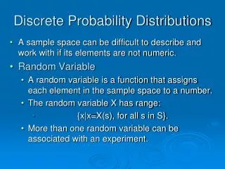
Random Variables RANDOM VARIABLE A quantity resulting from an experiment that, by chance, can assume different values.
CONTINUOUS RANDOM VARIABLE can assume an infinite number of values within a given range. It is usually the result of some type of measurement DISCRETE RANDOM VARIABLE A random variable that can assume only certain clearly separated values. It is usually the result of counting something. Types of Random Variables
DISCRETE RANDOM VARIABLE A random variable that can assume only certain clearly separated values. It is usually the result of counting something. Discrete Random Variables EXAMPLES • The number of students in a class. • The number of children in a family. • The number of cars entering a carwash in a hour. • Number of home mortgages approved by Coastal Federal Bank last week.
CONTINUOUS RANDOM VARIABLE can assume an infinite number of values within a given range. It is usually the result of some type of measurement Continuous Random Variables EXAMPLES • The length of each song on the latest Tim McGraw album. • The weight of each student in this class. • The temperature outside as you are reading this book. • The amount of money earned by each of the more than 750 players currently on Major League Baseball team rosters.
The Mean of a Probability Distribution • MEAN • The mean is a typical value used to represent the central location of a probability distribution. • The mean of a probability distribution is also referred to as its expected value (expectation), often written E(X). (We multiply each value by its probability and sum, exactly like we did for frequency distributions).
The Variance, and StandardDeviation of a Probability Distribution • Variance and Standard Deviation • Measures the amount of spread in a distribution • The computational steps are: • 1. Subtract the mean from each value, and square this difference. • 2. Multiply each squared difference by its probability. • 3. Sum the resulting products to arrive at the variance. • The standard deviation is found by taking the square root of the variance.
Mean, Variance, and StandardDeviation of a Probability Distribution - Example John Ragsdale sells new cars for Pelican Ford. John usually sells the largest number of cars on Saturday. He has developed the following probability distribution for the number of cars he expects to sell on a particular Saturday.
Variance and StandardDeviation of a Probability Distribution - Example So the main difference between what we did when we described data using frequency distributions and what we do now, is that we use probabilities instead of frequencies. We consider probabilities to be an intrinsic characteristic of a random variable, while frequencies may vary somewhat for each particular set of values it takes (a sample).
Class and Home Work p. 189, No. 1,3,5,7 in class No. 2,4,6,8 HW
Binomial Probability Distribution Characteristics of a Binomial Probability Distribution • There is a fixed number of ‘trials’ (like tosses of a coin). • Each trial can end in only one of 2 possible ways (head or tail, success or failure…) • The probability of a success is the same for all trials (the same is therefore true for the probability of a failure) • The trials are independent of each other • The random variable counts the number of successes over that fixed number of trials.
Binomial Probability Experiment • An outcome on each trial of an experiment is classified into one of two mutually exclusive categories—a success or a failure. • 2. The random variable counts the number of successes in a fixed number of trials. • 3. The probability of success and failure stay the same for each trial. • 4. The trials are independent, meaning that the outcome of one trial does not affect the outcome of any other trial.
Binomial Probability Formula n is the number of trials x is the number of observed successes π is the probability of success on each trial where nCx, often denoted Cnx, is
Binomial Probability - Example There are five flights daily from Pittsburgh via US Airways into the Bradford, Pennsylvania, Regional Airport. Suppose the probability that any flight arrives late is .20. What is the probability that none of the flights are late today?
Binomial Probability - Excel If you double-click on this, Excel will open and you’ll see all the formulas.
Binomial Dist. – Mean and Variance: Example For the example regarding the number of late flights, recall that =.20 and n = 5. What is the average number of late flights? What is the variance of the number of late flights?
Binomial Dist. – Mean and Variance: Another Solution A slight difference between the exact result of 0.80 and the value of s2 here is due to a round-off error.
Binomial Distribution - Table Five percent of the worm gears produced by an automatic, high-speed Carter-Bell milling machine are defective. What is the probability that out of six gears selected at random none will be defective? Exactly one? Exactly two? Exactly three? Exactly four? Exactly five? Exactly six out of six?
Binomial Distribution - MegaStat Five percent of the worm gears produced by an automatic, high-speed Carter-Bell milling machine are defective. What is the probability that out of six gears selected at random none will be defective? Exactly one? Exactly two? Exactly three? Exactly four? Exactly five? Exactly six out of six?
Binomial Distribution - Excel Excel can be used to find binomial probabilities. If you double-click on the table, Excel will open, and you’ll see the formulas. Here, it is useless to continue the table, because the probabilities of 16, 17 etc. successes are too small.
Binomial – Shapes for Varying (n constant) As p approaches 0.50, the distribution becomes symmetrical.
Binomial – Shapes for Varying n ( constant) As n grows, the distribution becomes more symmetrical.
Class and Home Work p. 197, No. 9,11,13,15,17 in class No. 10,12,14,16,18 HW
Binomial Probability Distributions - Example A study by the Illinois Department of Transportation concluded that 76.2 percent of front seat occupants used seat belts. A sample of 12 vehicles is selected. What is the probability the front seat occupants in exactly 7 of the 12 vehicles are wearing seat belts?
Cumulative Binomial Probability Distributions - Example A study by the Illinois Department of Transportation concluded that 76.2 percent of front seat occupants used seat belts. A sample of 12 vehicles is selected. What is the probability the front seat occupants in at least 7 of the 12 vehicles are wearing seat belts?
Cumulative Binomial Probability Distributions - Excel These calculations are very easy to do in Excel. The formula (in English) for the probability of 7 people wearing seat belts is =BINOMDIST(D11;12;0,762;0) where D11 contains 7, and the direct formula for the probability that at least 7 are wearing seat belts is =1-BINOMDIST(6;12;0,762;1).
Class and Home Work p. 199-200, No. 19,21,23 in class No. 20,22,24 HW
Poisson Probability Distribution • Now we do not have a fixed number of ‘trials’. • We have events occurring over intervals (mostly of time, but maybe of distance, volume…) with some frequency proportional to the size of the interval. • The intervals are independent: the number of events occurring in one interval does not affect the other intervals. • The random variable is the number of times the event occurs during a specified interval.
Poisson Probability Distribution The Poisson probability distribution is characterized by the number of times an event happens during some interval or continuum. Examples include: • The number of misspelled words per page in a newspaper. • The number of calls per hour received by Dyson Vacuum Cleaner Company. • The number of vehicles sold per day at Hyatt Buick GMC in Durham, North Carolina. • The number of goals scored in a college soccer game.
Poisson Probability Distribution • Sometimes we know the probabilitypof one event occurring, and the interval is measured as the number of trials, like in binomial distribution (but this number is not fixed). Then the average number of events during an interval of size nis m=np. • Sometimes we cannot interpret the interval as a number of trials, but we know that the frequency of the event is proportional to the size of the interval, and we know the meanm (the average number of events occurring during that interval).
Poisson Probability Distribution ThePoisson distribution can be described mathematically using the formula: The variance of Poisson distribution s2 = m.
Poisson Probability Distribution - Example Assume baggage is rarely lost by Northwest Airlines. Most flights have no lost bags; some have one, fewer have 2, and very seldom more. Suppose a random sample of 1000 flights shows a total of 300 bags were lost. Thus, the arithmetic mean of lost bags per flight it 0.3. If the number of lost bags per flight follows a Poisson distribution with m = 0.3, we can compute the various probabilities using the same formula. For example, the probability of losing no bags during a flight is and the probability of losing exactly one bag during one flight is
Poisson Probability Distribution - Table Recall from the previous illustration that the number of lost bags follows a Poisson distribution with a mean of 0.3. Use Appendix B.5 to find the probability that no bags will be lost on a particular flight. What is the probability exactly one bag will be lost on a particular flight?
More About the Poisson Probability Distribution • The Poisson probability distribution is always positively skewed and the random variable has no specific upper limit. • The Poisson distribution for the lost bags illustration, where µ=0.3, is highly skewed. As µ becomes larger, the Poisson distribution becomes more symmetrical.
Poisson Probability Distribution and Binomial Distribution A binomial distribution when the probability of success p is very small and the number of trials n is large, is difficult to distinguish from a Poisson distribution with the same mean (m = np).
Poisson Probability Distribution – example 3 Coastal Insurance Company underwrites insurance for beachfront properties. It uses the estimate that the probability of a hurricane hitting a particular region in any one year is 0.05. If a homeowner takes a 30-year mortgage on a recently purchased Property in that region, what is the probability he will experience at least one hurricane during the mortgage? p=0.05, n=30. We can solve this problem in two ways.
Poisson Probability Distribution – example 3, cont. p=0.05, n=30. Using Poisson Distribution: The average number of storms during a 30-year interval is m=np=300.5=1.5 Then P(at least one storm) = P(x 1) = 1 – P(x = 0)
Poisson Probability Distribution – example 3, cont. p=0.05, n=30. Using Binomial Distribution: yes, we can. There are 30 years, Each year is an independent trial (either a hurricane hits or it does not). We can practically exclude the possibility of more than one hurricane hitting the region during one year. So, we have the conditions of a Binomial Distribution. Then
Poisson Probability Distribution – example 3, cont. We get almost the same, but not quite the same, result: 0.7854 with the binomial approach, 0.7769 with the Poisson. You can think yourself which one is “more correct”. But anyway, they are almost the same. So I repeat: A binomial distribution when the probability of success p is very small and the number of trials n is large, is difficult to distinguish from a Poisson distribution with the same mean (m = np). And it is certainly easier to find the Poisson result.
Class and Home Work p. 208, No. 31,33,35 in class No. 32,34,36 HW, plus p.213, no. 62,66,70