Discrete Probability Distributions

1. Discrete Probability Distributions

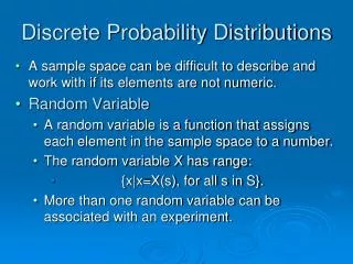
2. Random Variables • Random Variable (RV): A numeric outcome that results from an experiment • For each element of an experiment’s sample space, the random variable can take on exactly one value • Discrete Random Variable: An RV that can take on only a finite or countably infinite set of outcomes • Continuous Random Variable: An RV that can take on any value along a continuum (but may be reported “discretely” • Random Variables are denoted by upper case letters (Y) • Individual outcomes for RV are denoted by lower case letters (y)

3. Probability Distributions • Probability Distribution: Table, Graph, or Formula that describes values a random variable can take on, and its corresponding probability (discrete RV) or density (continuous RV) • Discrete Probability Distribution: Assigns probabilities (masses) to the individual outcomes • Continuous Probability Distribution: Assigns density at individual points, probability of ranges can be obtained by integrating density function • Discrete Probabilities denoted by: p(y) = P(Y=y) • Continuous Densities denoted by: f(y) • Cumulative Distribution Function: F(y) = P(Y≤y)

4. Discrete Probability Distributions

5. Example – Rolling 2 Dice (Red/Green) Y = Sum of the up faces of the two die. Table gives value of y for all elements in S

6. Rolling 2 Dice – Probability Mass Function & CDF

7. Rolling 2 Dice – Probability Mass Function

8. Rolling 2 Dice – Cumulative Distribution Function

9. Expected Values of Discrete RV’s • Mean (aka Expected Value) – Long-Run average value an RV (or function of RV) will take on • Variance – Average squared deviation between a realization of an RV (or function of RV) and its mean • Standard Deviation – Positive Square Root of Variance (in same units as the data) • Notation: • Mean: E(Y) = m • Variance: V(Y) = s2 • Standard Deviation: s

10. Expected Values of Discrete RV’s

11. Expected Values of Linear Functions of Discrete RV’s

12. Example – Rolling 2 Dice

13. Binomial Experiment • Experiment consists of a series of n identical trials • Each trial can end in one of 2 outcomes: Success (S) or Failure (F) • Trials are independent (outcome of one has no bearing on outcomes of others) • Probability of Success, p, is constant for all trials • Random Variable Y, is the number of Successes in the n trials is said to follow Binomial Distribution with parameters n and p • Y can take on the values y=0,1,…,n • Notation: Y~Bin(n,p)

14. Binomial Distribution

18. Poisson Distribution • Distribution often used to model the number of incidences of some characteristic in time or space: • Arrivals of customers in a queue • Numbers of flaws in a roll of fabric • Number of typos per page of text. • Distribution obtained as follows: • Break down the “area” into many small “pieces” (n pieces) • Each “piece” can have only 0 or 1 occurrences (p=P(1)) • Let l=np≡ Average number of occurrences over “area” • Y ≡ # occurrences in “area” is sum of 0s & 1s over “pieces” • Y ~ Bin(n,p) with p = l/n • Take limit of Binomial Distribution as n  with p = l/n

19. Negative Binomial Distribution • Used to model the number of trials needed until the rth Success (extension of Geometric distribution) • Based on there being r-1 Successes in first y-1 trials, followed by a Success

20. Negative Binomial Distribution (II) This model is widely used to model count data when the Poisson model does not fit well due to over-dispersion: V(Y) > E(Y). In this model, k is not assumed to be integer-valued and must be estimated via maximum likelihood (or method of moments)