Download
1 / 21
210 likes | 387 Views
Scalar Mixing in Turbulent, Confined Axisymmetric Co-flows. C.N. Markides & E. Mastorakos Hopkinson Laboratory, Department of Engineering Monday, 6 th of February, 2006. 1/19. The Turbulent, Confined Axisymmetric Co-flow 1.

E N D
Scalar Mixing inTurbulent, ConfinedAxisymmetric Co-flows C.N. Markides & E. Mastorakos Hopkinson Laboratory, Department of Engineering Monday, 6th of February, 2006
1/19 The Turbulent, ConfinedAxisymmetric Co-flow1 • Axisymmetric flow configuration (r,z) • Dimensions: • Quartz tube inner Ø D=33.96mm • Injector outer Ø do=2.975mm • Injector inner Ø d=2.248mm and 1.027mm • Domain (laser sheet) height 60mm • Co-flow air preheated to 200±1oC • Upstream (63mm from injector nozzle) perforated grid (M=3mm circular holes, 44% solidity) enhances co-flow turbulence level • Injected stream: • Begins as nitrogen-diluted fuel • YC2H2=0.73 C2H2/N2 or YH2=0.14 H2/N2 • Passes though seeder that introduces 20% acetone b.v. • For co-flow define: • Reco = UcoM/ν, or, Returb = u'coLturb/ν • Reco range: 395-950; ***Returb≈Reco/10*** • For injected stream define: • υinj=Uinj/Uco • υinj range: 1.1-4.9; ***Not a free jet*** • δinj= ρinj/ρco • δinj=1.2 forC2H2/N2/acetone • δinj=0.8 for H2/N2/acetone Laser Sheet Fuel Injection z Uinj, Tinj r Injector Quartz Tube Uco, Tco Air from MFC Acetone Seeded Fuel Grid 1. See Markides and Mastorakos (2005) in Proc. Combust. Inst.; Markides (2006) Ph.D. Thesis; Markides, De Paola and Mastorakos (2006) shortly in Exp. Therm. Fluid Sci. for details.
2/19 Planar Laser-Induced Fluorescence Measurements (Brief Overview2) • Each ‘Run’ corresponds to a set of fixed Uco, Uinj and Yfuel conditions (i.e. Reco/Returb, υinj and δfuel) • The raw measurements are near-instantaneous (integrated over 0.4μs) images of size (height x width) 1280 x 480 pixels • For each ‘Run’ we generated 200 images at 10Hz (every 0.1s) • Images are 2-dimensional planar measurements: • Smallest lengthscale in the flow is Kolmogorov (ηK) and was measured at 0.2-0.3mm • Laser-sheet thickness (spatial resolution) ≈ 0.10±0.03mm • Measured intensity at any image pixel is the spatial average over a square region of length 0.050-0.055mm at that point in the flow • Ensemble spatial resolution is 0.09mm • Ability to transfer contrast information quantified by Modulation Transfer Function (MTF). Investigation revealed ability to resolve 70-80% of spatial detail with 4-5 pixels or 0.3mm • Local intensity proportional to local volumetric/molar concentration of acetone vapour, so that: • Convert to mass-based mixture fraction by: • Two-dimensional scalar dissipation (the Greek one - χ) was calculated by: ***But before this was done the images of ξ were filtered and denoised*** 2. See Markides and Mastorakos (2006) in Chem. Eng. Sci.; Markides (2006) Ph.D. Thesis for details.
3/19 Quantifying Measurement Resolution
4/19 Obtaining the instantaneous χ2D field from the instantaneous ξ field (I) ξ χ2D
5/19 Obtaining the instantaneous χ2D field from the instantaneous ξ field (II) ξ χ2D
6/19 Obtaining the instantaneous χ2D field from the instantaneous ξ field (III) ξ χ2D
7/19 Obtaining the instantaneous χ2D field from the instantaneous ξ field (IV) • At this stage have considered the squares of the spatial gradients of ξ, (∂ξ/∂r)2 and (∂ξ/∂z)2; we also have the spatial gradients of ξ', (∂ξ'/∂r)2 and (∂ξ'/∂z)2 • Finally, need molecular diffusivity (D): • Consider ternary (acetone-’1’, nitrogen-’2’ and fuel-’3’) diffusion coefficients from binary diffusion coefficients (D11, D12, D13, D22, D23, D33) • Simplify by assuming that D12≈D13 or X1<<1 so that D12T<<D11T and calculate D1,mix at each point in the flow, given that we already have the instantaneous X1 (from ξ)
8/19 Calculating Mixing Quantities (I) • For each ‘Run’ and at each pixel representing a location in physical space (r,z) loop through 200 images: • Of each version of ξ (raw and all stages of processing) to obtain the mean and variance of each version of ξ • Of each version of corresponding (∂ξ/∂r)2 and (∂ξ/∂z)2 to obtain the mean and variance of each version of (∂ξ/∂r)2 and (∂ξ/∂z)2 • Of each version of corresponding (∂ξ'/∂r)2 and (∂ξ'/∂z)2 to obtain the mean and variance of each version of (∂ξ'/∂r)2 and (∂ξ'/∂z)2 • Evaluate spatial 2-point autocorrelation matrices along centreline and at left/right half-widths • Compile radial volume-averaged quantities (i.e. at one z group all r data together)
9/19 Calculating Mixing Quantities (II) • For each ‘Run’ and at each pixel representing a location in physical space (r,z) consider a window of size 1x1 (or 2x10) ηK containing 40 (or 720) pixels and loop through 200 images: • At 15 axial locations from 1mm to 60mm in steps of 4mm • At 5 radial locations with r=0, ±d/2, ±d • Calculate the local mean, variance, skewness and kurtosis of all versions of all variables (ξ and χ2D) • Calculate the local mean, variance, skewness and kurtosis of the logarithm of all versions of χ2D • Compile pdfs of all versions of all variables (ξ and χ2D) each composed of 90 and 30 points respectively spanning the min-max range (from about 140,000 data points) • Separate the χ2D data into 30 groups between the min-max range of ξ by considering the corresponding values of ξ (χ2D|ξ) • Calculate the local mean, variance, skewness and kurtosis of χ2D|ξ and ln(χ2D|ξ) • Compile pdfs of all versions of χ2D|ξ: • unless number of data points in the local pdf is less than 300 • each composed of 30 points respectively spanning the min-max range • from about 2,000-10,000 data points
10/19 Below: All are equal velocity cases (Uinj≈Uco; υinj=1.0±0.2) with the 2.248mm injector and varying Reco/Returb Right: Jet cases with the 2.248mm injector (υinj=3 and 4) Not affected by image processing Mean ξ (I)
11/19 Mean ξ (II)
12/19 Variance of ξ (I) • Left: • Equal velocity case • Right: • Jet case • Affected by image processing
13/19 Variance of ξ (II)
14/19 Mean χ2D (I) • Equal velocity case • Significantly affected by image processing
15/19 Mean χ2D (II)
16/19 (Non-strict) Isotropy in χ2D
17/19 Mean Scalar Dissipation Modelling and CD (I) • At each location in physical space where we would like to evaluate: • Firstly we need to recover the mean full 3-dimensional χ from the mean χ2D (along the centreline by symmetry the mean gradients squared in the radial and azimuthal direction are equal) • Also examined isotropy of the two components • We also need knowledge of the turbulent timescale (k/ε) where k is the turbulence kinetic energy and ε the mean turbulence dissipation • Use (k/ε)/(Lturb/u')≈1.7±0.2 Pope (2000)
18/19 Mean Scalar Dissipation Modelling and CD (II) Centreline U/Uco (z+63mm)/d Centreline u'/Uco (z+63mm)/d
19/19 Mean Scalar Dissipation Modelling and CD (III) τturb/τturb(z/d=35)
Scalar Mixing inTurbulent, ConfinedAxisymmetric Co-flows C.N. Markides & E. Mastorakos Hopkinson Laboratory, Department of Engineering Monday, 6th of February, 2006