Download
1 / 21
210 likes | 306 Views
Initialization of Land-Surface Schemes for Subseasonal Predictions. Paul Dirmeyer. Soil moisture decorrelation time-scales. Land surface “memory” is concentrated in the sub-seasonal time-scale (0-3 months).

E N D
Initialization of Land-Surface Schemes for Subseasonal Predictions. Paul Dirmeyer
Soil moisture decorrelation time-scales • Land surface “memory” is concentrated in the sub-seasonal time-scale (0-3 months). • Land surface “memory” is an ideal piece of potential predictability to be harvested for sub-seasonal forecasts.
Goal of land initialization • Consistency across models (same anomalies) • Consistency within model (between initial land state and land model)
Sources of initialization • Observations • Independent data sets (from a different model than yours) • Consistent offline data set (from your land model) • Coupled LDAS (your land and atmosphere models)
Combine meteorological observations (forcings) with a model of the land surface: • Mintz and Serafini • Schemm et al. • Schnur and Lettenmaier • Willmott and Matsura • Huang et al. • Dirmeyer and Tan (GOLD) • Current Land Data Assimilation System (LDAS) products Independent data sets
Huang and van den Dool Independent data sets NCEP/CPC
Land Data Assimilation System (LDAS) – no assimilation Independent data sets N-LDAS
Independent data sets • All have a basic shortcoming – the product is from someone else’s model • Soil wetness is not easily transferable between models. Koster and Milly
Consistent offline data set • Global Soil Wetness Project (GSWP) • Historical • Land Data Assimilation System (LDAS) • Real Time Uses observed/analysis meteorological forcing to drive your land model uncoupled from atmospheric model. Generates land surface state variables and fluxes for best-possible atmosphere, but without feedback processes. True LDAS will also assimilate land surface state variable observations.
Global Soil Wetness Project (GSWP) • Your model must be in the project to generate the initial conditions. COLA/SSIB
US (North American and Global)-LDAS approach: • Assimilation of observations of soil temperature and moisture • Strictly uncoupled from atmosphere • Multi-model LDAS Approaches
evaporation Boundary layer scheme Observations driving soil moisture correction METEOSAT/MSG AMSR (?) Synops data precipitation radiation Soil moisture content Land surface parameterization scheme Soil moisture correction scheme (sub)surface runoff LDAS Approaches • European-LDAS approach: • Relaxation of coupled PBL to observations • Assimilation of observations to nudge soil moisture • Multi-model
Coupled LDAS • Land model is coupled to its parent atmospheric model during integration. • Shortcomings of atmospheric model fluxes (precipitation, radiation…) are overcome by some intervention: • Replace downward fluxes (poor-man’s LDAS) • Flux adjustment (similar to ocean-atmosphere) • Empirical correction of state variables
ATMOSPHERIC CALCULATIONS Time step n+1 ATMOSPHERIC CALCULATIONS Time step n E,H E,H Precip. Precip. Rad. Rad. T,q,… T,q,… Observed Precip. Observed Precip. LAND CALCULATIONS Time step n LAND CALCULATIONS Time step n+1 POOR MAN’S LDAS: A study of the impacts of soil moisture initialization on seasonal forecasts At every time step in a GCM simulation, the land surface model is forced with observed precipitation rather than GCM-generated precipitation. The observed global daily precipitation data comes from GPCP and covers the period 1997-2001 at a resolution of 1o X 1o (George Huffman, pers. Comm.) The daily precipitation is applied evenly over the day.
Compromises • None of the above methods combine the key elements necessary for initialization of a broad, voluntary, multi-model experiment: • Easy • Cheap • Fast
Compromises • Possible Solution: • Composite soil wetness: • Interannual anomalies from an agreed-upon quasi-observed product • Mean annual cycle from your land model (e.g., from AMIP-2, C20C, etc.)
Key questions: • How to scale the soil wetness (and snow) anomalies to be consistent with your model? • Water mass – but soil capacities may not agree Compromises
Compromises • A better solution: • Interannual standard deviation* Standard normal deviates: but AMIP coupled L-A variance may be poor March 1, 2002 soil wetness anomaly (percent of saturation) for a) Huang et al. (1996) and b) COLA GCM initial condition. * Origins of the Summer 2002 Continental U.S. Drought M. J. Fennessy, P. A. Dirmeyer, J. L. Kinter III, L. Marx and C. A. Schlosser 2002 Climate Diagnostics and Prediction Workshop, Vienna, VA.
Vegetation • Good estimates of vegetation phenology exist from remote sensing (NDVI → LAI, Greenness). • Hindcast: climatology versus observed • Forecast: climatology versus persisted anomaly