Download
1 / 61
610 likes | 613 Views
Topic 1b: Flow Analysis. Some slides come from Prof. J. N. Amaral (amaral@cs.ualberta.ca). Motivation Control flow analysis Dataflow analysis Advanced topics. Topic 4: Flow Analysis. Slides Dragon book: chapter 8.4, 8.5, Chapter 9 Muchnick’s book: Chapter 7

E N D
Topic 1b: Flow Analysis Some slides come from Prof. J. N. Amaral (amaral@cs.ualberta.ca) \course\cpeg421-10F\Topic1-b.ppt
Motivation Control flow analysis Dataflow analysis Advanced topics Topic 4: Flow Analysis \course\cpeg421-10F\Topic1-b.ppt
Slides Dragon book: chapter 8.4, 8.5, Chapter 9 Muchnick’s book: Chapter 7 Other readings as assigned in class or homework Reading List \course\cpeg421-10F\Topic1-b.ppt
Flow Analysis Control flow analysis Interprocedural Program Intraprocedural Procedure Flow analysis Data flow analysis Local Basic block • Control Flow Analysis─ Determine control structure of a program and build a Control Flow Graph. • Data Flow analysis ─ Determine the flow of scalar values and ceretain associated properties • Solution to the Flow analysis Problem: propagation of data flow information along a flow graph. \course\cpeg421-10F\Topic1-b.ppt
Code optimization - a program transformation that preserves correctness and improves the performance (e.g., execution time, space, power) of the input program. Code optimization may be performed at multiple levels of program representation: 1. Source code 2. Intermediate code 3. Target machine code Optimized vs. optimal - the term “optimized” is used to indicate a relative performance improvement. Introduction to Code Optimizations \course\cpeg421-10F\Topic1-b.ppt
Motivation S1: A 2 (def of A) S2: B 10 (def of B) S3: C A + B determine if C isaconstant 12? S4 Do I = 1, C A[I] = B[I] + D[I-1] . . . \course\cpeg421-10F\Topic1-b.ppt
Basic Blocks Only the last statement of a basic block can be a branch statement and only the first statement of a basic block can be a target of a branch. However, procedure calls may need be treated with care within a basic block (Procedure call starts a new basic block) A basic block is a sequence of consecutive intermediate language statements in which flow of control can only enter at the beginning and leave at the end. (AhoSethiUllman, pp. 529) \course\cpeg421-10F\Topic1-b.ppt
1. Identify leader statements (i.e. the first statements of basic blocks) by using the following rules: (i) The first statement in the program is a leader (ii) Any statement that is the target of a branch statement is a leader (for most IL’s. these are label statements) (iii) Any statement that immediately follows a branch or return statement is a leader 2. The basic block corresponding to a leader consists of the leader, and all statements up to but not including the next leader or up to the end of the program. Basic Block Partitioning Algorithm \course\cpeg421-10F\Topic1-b.ppt
Example The following code computes the inner product of two vectors. • (1) prod := 0 • (2) i := 1 • (3) t1 := 4 * i • (4) t2 := a[t1] • (5) t3 := 4 * i • (6) t4 := b[t3] • (7) t5 := t2 * t4 • (8) t6 := prod + t5 • (9) prod := t6 • (10) t7 := i + 1 • (11) i := t7 • if i <= 20 goto (3) • (13) … begin prod := 0; i := 1; do begin prod := prod + a[i] * b[i] i = i+ 1; end while i <= 20 end Source code. Three-address code. \course\cpeg421-10F\Topic1-b.ppt
Example The following code computes the inner product of two vectors. (1) prod := 0 (2) i := 1 (3) t1 := 4 * i (4) t2 := a[t1] (5) t3 := 4 * i (6) t4 := b[t3] (7) t5 := t2 * t4 (8) t6 := prod + t5 (9) prod := t6 (10) t7 := i + 1 (11) i := t7 (12) if i <= 20 goto (3) (13) … Rule (i) begin prod := 0; i := 1; do begin prod := prod + a[i] * b[i] i = i+ 1; end while i <= 20 end Source code. \course\cpeg421-10F\Topic1-b.ppt Three-address code.
Example The following code computes the inner product of two vectors. Rule (i) (1) prod := 0 (2) i := 1 (3) t1 := 4 * i (4) t2 := a[t1] (5) t3 := 4 * i (6) t4 := b[t3] (7) t5 := t2 * t4 (8) t6 := prod + t5 (9) prod := t6 (10) t7 := i + 1 (11) i := t7 (12) if i <= 20 goto (3) (13) … begin prod := 0; i := 1; do begin prod := prod + a[i] * b[i] i = i+ 1; end while i <= 20 end Rule (ii) Source code. \course\cpeg421-10F\Topic1-b.ppt Three-address code.
Example The following code computes the inner product of two vectors. (1) prod := 0 (2) i := 1 (3) t1 := 4 * i (4) t2 := a[t1] (5) t3 := 4 * i (6) t4 := b[t3] (7) t5 := t2 * t4 (8) t6 := prod + t5 (9) prod := t6 (10) t7 := i + 1 (11) i := t7 (12) if i <= 20 goto (3) (13) … Rule (i) begin prod := 0; i := 1; do begin prod := prod + a[i] * b[i] i = i+ 1; end while i <= 20 end Rule (ii) Rule (iii) Source code. \course\cpeg421-10F\Topic1-b.ppt Three-address code.
Example B1 (1) prod := 0 (2) i := 1 (3) t1 := 4 * i (4) t2 := a[t1] (5) t3 := 4 * i (6) t4 := b[t3] (7) t5 := t2 * t4 (8) t6 := prod + t5 (9) prod := t6 (10) t7 := i + 1 (11) i := t7 (12) if i <= 20 goto (3) B2 Basic Blocks: B3 (13) … \course\cpeg421-10F\Topic1-b.ppt
Transformations on Basic Blocks • Structure-Preserving Transformations: • common subexpression elimination • dead code elimination • renaming of temporary variables • interchange of two independent adjacent statements • Others … \course\cpeg421-10F\Topic1-b.ppt
Transformations on Basic Blocks The DAG representation of a basic block lets compiler perform the code-improving transformations on the codes represented by the block. \course\cpeg421-10F\Topic1-b.ppt
Transformations on Basic Blocks Algorithm of the DAG construction for a basic block • Create a node for each of the initial values of the variables in the basic block • Create a node for each statement s, label the node by the operator in the statement s • The children of a node N are those nodes corresponding to statements that are last definitions of the operands used in the statement associated with node N. Tiger book pp533 \course\cpeg421-10F\Topic1-b.ppt
An Example of Constructing the DAG Step (1): create node 4 and i0 Step (2): create node * Step (3): attach identifier t1 Step (1): create nodes labeled [], a Step (2): find previously node(t1) Step (3): attach label Here we determine that: node (4) was created node (i) was created node (*) was created t1: = 4*i t2 := a[t1] t3 := 4*i t1 * 4 i0 t2 [ ] t1,t3 a0 * just attach t3 to node * 4 i0 \course\cpeg421-10F\Topic1-b.ppt
Example of Common Subexpression Elimination c + a:= b + c b:= a – d c:= b + c d:= b • a:= b + c • b:= a – d • c:= b + c • d:= a - d Detection: Common subexpressions can be detected by noticing, as a new node m is about to be added, whether there is an existing node n with the same children, in the same order, and with the same operator. if so, n computes the same value as m and may be used in its place. b,d - a d0 + c0 b0 If a node N represents a common subexpression, N has more than one attached variables in the DAG. \course\cpeg421-10F\Topic1-b.ppt
Example of Dead Code Elimination if x is never referenced after the statement x = y+z, the statement can be safely eliminated. \course\cpeg421-10F\Topic1-b.ppt
Example of Renaming Temporary Variables rename (1) t := b + c (1) u := b + c t u Change (rename) label + + b0 c0 b0 c0 if there is an statement t := b + c, we can change it to u := b + c and change all uses of t to u. a code in which each temporary is defined only once is called a single assignment form. \course\cpeg421-10F\Topic1-b.ppt
t1 := b + c t2 := x + y Observation: We can interchange the statements without affecting the value of the block if and only if neither x nor y is t1 and neither b nor c is t2, i.e. we have two DAG subtrees. Example of Interchange of Statements t1 t2 + + b0 c0 x0 y0 \course\cpeg421-10F\Topic1-b.ppt
Arithmetic Identities: x + 0 = 0 + x = x x – 0 = x x * 1 = 1 * x = x x / 1 = x - Replace left-hand side with simples right hand side. Associative/Commutative laws x + (y + z) = (x + y) + z x + y = y + x Reduction in strength: x ** 2 = x * x 2.0 * x = x + x x / 2 = x * 0.5 - Replace an expensive operator with a cheaper one. Constant folding 2 * 3.14 = 6.28 -Evaluate constant expression at compile time` Example of Algebraic Transformations \course\cpeg421-10F\Topic1-b.ppt
A control flow graph (CFG), or simply a flow graph, is a directed multigraph in which the nodes are basic blocks and edges represent flow of control (branches or fall-through execution). •The basic block whose leader is the first statement is called the initial node or start node • There is a directed edge from basic block B1 to basic B2 in the CFG if: (1) There is a branch from the last statement of B1 to the first statement of B2, or (2) Control flow can fall through from B1 to B2 because B2 immediately follows B1, and B1 does not end with an unconditional branch Control Flow Graph (CFG) And, there is an END node. \course\cpeg421-10F\Topic1-b.ppt
Example (1) prod := 0 (2) i := 1 B1 Control Flow Graph: Rule (2) (3) t1 := 4 * i (4) t2 := a[t1] (5) t3 := 4 * i (6) t4 := b[t3] (7) t5 := t2 * t4 (8) t6 := prod + t5 (9) prod := t6 (10) t7 := i + 1 (11) i := t7 (12) if i <= 20 goto (3) B2 B1 B2 B3 Rule (1) Rule (2) B3 (13) … \course\cpeg421-10F\Topic1-b.ppt
CFGs are Multigraphs Note: there may be multiple edges from one basic block to another in a CFG. Therefore, in general the CFG is a multigraph. The edges are distinguished by their condition labels. A trivial example is given below: [101] . . . [102] if i > n goto L1 Basic Block B1 False True [103] label L1: [104] . . . Basic Block B2 \course\cpeg421-10F\Topic1-b.ppt
Identifying loops Question: Given the control flow graph of a procedure, how can we identify loops? Answer: We use the concept of dominance. \course\cpeg421-10F\Topic1-b.ppt
Dominators Node (basic block) D in a CFG dominatesnode N if every path from the start node to N goes through D. We say that node D is a dominator of node N. Define DOM(N) = set of node N’s dominators, or the dominator set for node N. Note: by definition, each node dominates itself i.e., N DOM(N). \course\cpeg421-10F\Topic1-b.ppt
Domination Relation Definition: Let G= (N, E, s) denote a flowgraph. and let n, n’ N. 1. ndominatesn’, written n n’ : each path from s to n’ contains n. 2. nproperly dominatesn’, written n < n’ : n n’ and n n’. 3. ndirectly (immediately) dominatesn’, written n <d n’: n < n’ and there is no m N such that n < m < n’. 4. DOM(n) := {n’ : n’ n} is the set of dominators of n. \course\cpeg421-10F\Topic1-b.ppt
Domination Property • The domination relation is a partial ordering • Reflexive A A • Antisymmetric A B B A • Transitive A B and B C A C \course\cpeg421-10F\Topic1-b.ppt
Computing Dominators Observe: if a dominates b, then • a = b, or •a is the only immediate predecessor of b, or •b has more than one immediate predecessor, all of which are dominated by a. DOM(b) = {b} U ∩ DOM(p) p pred(b) Quiz: why here is the intersection operator instead of the union? \course\cpeg421-10F\Topic1-b.ppt
An Example Domination relation: { (1, 1), (1, 2), (1, 3), (1, 4) … (2, 3), (2, 4), … (2, 10) ... } S 1 2 3 Direct domination: 4 1 <d 2, 2 <d 3, … 5 6 7 DOM: 8 DOM(1) = {1} DOM(2) = {1, 2} DOM(10) = {1, 2, 10} … 9 10 DOM(8) ? DOM(8) ={ 1,2,3,4,5,8} \course\cpeg421-10F\Topic1-b.ppt
Question Assume node m is an immediate dominator of a node n, is mnecessarily an immediate predecessor of n in the flow graph? S 1 2 3 4 5 6 7 Answer: NO! Example: consider nodes 5 and 8. 8 9 10 \course\cpeg421-10F\Topic1-b.ppt
Dominance Intuition S Imagine a source of light at the start node, and that the edges are optical fibers 1 2 3 4 5 To find which nodes are dominated by a given node a, place an opaque barrier at a and observe which nodes became dark. 6 7 8 9 10 \course\cpeg421-10F\Topic1-b.ppt
Dominance Intuition S The start node dominates all nodes in the flowgraph. 1 2 3 4 5 6 7 8 9 10 \course\cpeg421-10F\Topic1-b.ppt
Dominance Intuition S 1 Which nodes are dominated by node 3? 2 3 4 5 6 7 8 9 10 \course\cpeg421-10F\Topic1-b.ppt
Dominance Intuition S 1 Which nodes are dominated by node 3? 2 3 4 Node 3 dominates nodes 3, 4, 5, 6, 7, 8, and 9. 5 6 7 8 9 10 \course\cpeg421-10F\Topic1-b.ppt
Dominance Intuition S 1 Which nodes are dominated by node 7? 2 3 4 5 6 7 8 9 10 \course\cpeg421-10F\Topic1-b.ppt
Dominance Intuition S 1 Which nodes are dominated by node 7? 2 3 4 5 Node 7 only dominates itself. 6 7 8 9 10 \course\cpeg421-10F\Topic1-b.ppt
Node Mis the immediate dominator of node N==> Node M must be the last dominator of N on any path from the start node to N. Therefore, every node other than the start node must have a unique immediate dominator (the start node has no immediate dominator.) Immediate Dominators and Dominator Tree What does this mean ? \course\cpeg421-10F\Topic1-b.ppt
A Dominator Tree A dominator tree is a useful way to represent the dominance relation. In a dominator tree the start node s is the root, and each node d dominates only its descendants in the tree. \course\cpeg421-10F\Topic1-b.ppt
S 1 2 1 3 2 4 10 3 5 4 6 7 5 9 8 7 8 6 9 10 Dominator Tree (Example) A flowgraph (left) and its dominator tree (right) \course\cpeg421-10F\Topic1-b.ppt
• Back-edges - an edge (B, A), such that A < B (A properly dominates B). • Header --A single-entry node which dominates all nodes in a subgraph. • Natural loops: given a back edge (B, A), a natural loop of (B, A) with entrynode A is the graph: A plus all nodes which is dominated by A and can reach B without going through A. Natural Loops \course\cpeg421-10F\Topic1-b.ppt
Find Natural Loops One way to find natural loops is: start 1) find a back edge (b,a) 2) find the nodes that are dominated by a. a 3) look for nodes that can reach bamong the nodes dominated bya. b \course\cpeg421-10F\Topic1-b.ppt
Algorithm to finding Natural Loops Input: A flow graph G and a back edge n -> d Output: the natural loop of n ->d • Initial a loop L with nodes n and d: L={n, d}; • Mark d as “visible” so that the following search does not reach beyond d; • Perform a depth-first search on the control-flow graph starting with node n; • Insert all the nodes visited in this search into loop L. - Alg. 9.46 (Aho et. al., pp665) \course\cpeg421-10F\Topic1-b.ppt
(9,1) An Example Find all back edges in this graph and the natural loop associated with each back edge 1 2 3 Back edge Natural loop 4 6 5 7 8 10 9 \course\cpeg421-10F\Topic1-b.ppt
An Example Find all back edges in this graph and the natural loop associated with each back edge 1 2 3 Back edge Natural loop (9,1) Entire graph 4 6 5 7 8 10 9 \course\cpeg421-10F\Topic1-b.ppt
(10,7) An Example Find all back edges in this graph and the natural loop associated with each back edge 1 2 3 Back edge Natural loop (9,1) Entire graph 4 6 5 7 8 10 9 \course\cpeg421-10F\Topic1-b.ppt
(10,7) An Example Find all back edges in this graph and the natural loop associated with each back edge 1 2 3 Back edge Natural loop (9,1) Entire graph 4 6 5 7 8 10 9 \course\cpeg421-10F\Topic1-b.ppt
An Example Find all back edges in this graph and the natural loop associated with each back edge 1 2 3 Back edge Natural loop (9,1) Entire graph 4 (10,7) {7,8,10} 6 5 7 8 10 9 \course\cpeg421-10F\Topic1-b.ppt
(7,4) An Example Find all back edges in this graph and the natural loop associated with each back edge 1 2 3 Back edge Natural loop (9,1) Entire graph 4 (10,7) {7,8,10} 6 5 7 8 10 9 \course\cpeg421-10F\Topic1-b.ppt