5-1 HOMOGENEOUS PRODUCTION FUNCTION

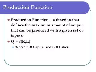
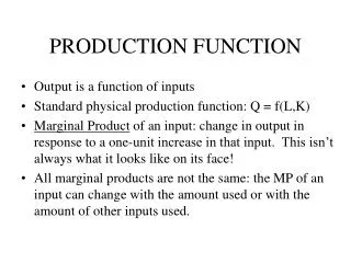
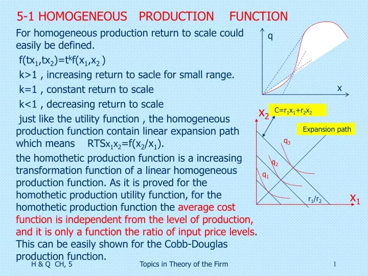
1. q 5-1 HOMOGENEOUS PRODUCTION FUNCTION C=r1x1+r2x2 x q3 x2 q2 Expansion path For homogeneous production return to scale could easily be defined. f(tx1,tx2)=tkf(x1,x2 ) k>1 , increasing return to sacle for small range. k=1 , constant return to scale k<1 , decreasing return to scale just like the utility function , the homogeneous production function contain linear expansion path which means RTSx1x2=f(x2/x1). the homothetic production function is a increasing transformation function of a linear homogeneous production function. As it is proved for the homothetic production utility function, for the homothetic production function the average cost function is independent from the level of production, and it is only a function the ratio of input price levels. This can be easily shown for the Cobb-Douglas production function. q1 r1/r2 x1 Topics in Theory of the Firm

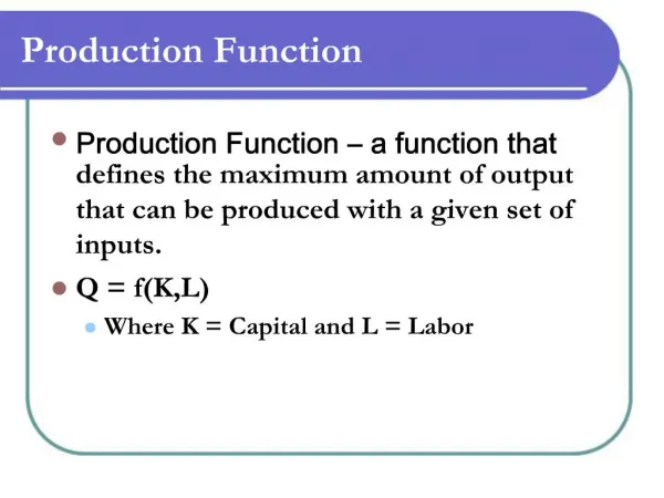
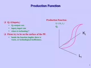
2. 5-1 HOMOGENEOUS PRODUCTION FUNCTION q=f(x1,x2) If f(tx1,tx2) = tkf(x1,x2) , then x1f1 + x2f2 = kf(x1 , x2) If k=1 , then x1f1 + x2f2 = q = f(x1 , x2) (x1f1)/q + (x2f2)/q = 1 (∂q/ ∂x1)(x1/q) + (∂q/ ∂x2)(x2/q) =1 єx1,q + єx2,q =1 exhaustion theorem , or x1f1 + x2f2 = q marginal productivity theory of distribution two steps ; 1 – each factor should receive its marginal productivity 2 – all output should be exhausted. for k=1, long run profit equals to zero. Π=pq – r1x1 – r2x2 = pq – pf1x1–pf2x2 = pq –p(f1x1 + f2x2)=pq – pq =0 Π(t)=pf(tx1,tx2) – r1tx1 – r2tx2 =t pf(x1,x2) –tr1x1– tr2x2 =tΠ profit function is homogenous of degree one with respect to scale of production. If each factor is paid according to it’s value of marginal product , profit will be zero regardless of its scale of production. Topics in Theory of the Firm

3. 5-1 HOMOGENEOUS PRODUCTION FUNCTION So when production function is homogeneous of degree one, the scale of production is not defined; If Π>0 , t (scale of production) can be increased forever. If Π<0 the firm will go out of business. If Π=0 scale can not be defined. Solution ; In order to use the exhaustion theorem results, considering the above difficulties; 1 –Production function defined not as homogeneous of degree one. 2- First and second order condition for profit maximization should exist. 3- maximum profit should equal to zero . Π=pq – r1x1– r2x2 =0 , r1=pf1 , r2=pf2 , Π=pq– pf1x1–pf2x2 =0 , q=f1x1+f2x2 (exhaustion theorem) undefined scale of production, actually means non existence of the second order condition for profit maximization. Topics in Theory of the Firm

4. 5-1 HOMOGENEOUS PRODUCTION FUNCTION x1f1 + x2f2 =q (f1+x1f11+x2f21)dx1 + (f2 + x1f12 + x2f22 )dx2 = dq dq/dx1(dx2=0)=f1+f11x1 +x2f21=f1 , f11 = (-x2/x1)f21 dq/dx2(dx1=0)=f2+f22x2 +x1f12=f2 , f22 = (-x1/x2)f12 f11f22–f122= f122 - f122 = 0(straight line.It should be greater than zero). However, constant return to scale assumption is needed in many cases; what should be done; we assume that 1-, the whole industry has a constant return to scale production function but the individual firm does not. 2-Scale of production is finite, in such a way that equates demand with supply in the whole industry . The long run cost function will have a special shape when production function is homogeneous . Suppose that x10 and x20 , relates to the one unit of the production level f(tx10,t x20)=tkf(x10,x20)=tk , so; q=tk c=r1x10 + r2x20 =a → cost of producing one unit Topics in Theory of the Firm

5. 5-1 HOMOGENEOUS PRODUCTION FUNCTION C=at total cost of producing q units. q=tk production function , C=aq1/k total cost function , AC = TC/q= aq(1-k)/k , MC=(a/k)q(1-k)/k 5-2 C.E.S. PRODUCTION FUNCTION An special form of homogeneous production function is the one which has Constant Elasticity of Substitution. q=A[αx1-ρ + (1-α)x2 -ρ ]-1/ ρ homogeneous of degree one. MPx1=(∂q/∂x1) =[α/(A-ρ)](q/x1) ρ+1 homogeneous of degree zero MPx2=(∂q/∂x2) =[(1-α)/(A-ρ)](q/x2) ρ+1 homogeneous of degree zero RTSx1 x2 =( MPx1)/( MPx2)=[α/(A-ρ)](q/x1) ρ+1/[(1-α)/(A-ρ)](q/x2) ρ+1 RTSx1 x2=[α/(1-α)](x2/x1) ρ+1 , if x1 increases then RTS wil decrease σ=(f1f2)/(f12q) , f12={(ρ+1) α (1-α)q2ρ+1}/A2ρ , σ=1/(ρ+1) , ρ=(1- σ)/ σ since σ>0 , then ρ>-1 for concavity condition to prevail. Topics in Theory of the Firm

6. x2 RTS= ∞ RTS=0 5-2 C.E.S. PRODUCTION FUNCTION x1 1 – if σ 0 then ρ ∞ , RTS= =[α/(1-α)](x2/x1) ρ+1 when ρ ∞, if x2>x1 , RTS = ∞ , if x1>x2 , RTS =0 2 – 0< σ<1 , ρ > 0 q=A[αx1-ρ + (1-α)x2 -ρ ]-1/ ρ If q=q0 , then , αx1-ρ + (1-α)x2 -ρ = q0/A = K If x1=0 , x2 is not defined, if x1 ∞, αx1-ρ =0 , x2=[K/(1- α)]-1/ρ If x2=0 , x1 is not defined, if x2 ∞, (1-α)x2 -ρ =0 , x1=(K/α)-1/ρ x2 [K/(1- α)]-1/ρ=x2 x1 x1=(K/α)-1/ρ Topics in Theory of the Firm

7. 5-2 C.E.S. PRODUCTION FUNCTION x2=[K/(1- α)]-ρ 3 – if σ =1, ρ=0, q is not defined, using hopital rule we get Cobb-Douglass production function 4 – if σ>1, , -1< ρ <0 , αx1-ρ + (1-α)x2 -ρ = q0/A = K if x1=0 , then , x2=[K/(1- α)]-ρ if x2=0 , then , x1=(K/α)-ρ 5 – σ ∞ , then ρ -1 , αx1 + (1-α)x2 = q0/A = K if x1=0 , then , x2=[K/(1- α)] if x2=0 , then , x1=(K/α) x1=(K/α)-ρ x2=[K/(1- α)] x1=(K/α) Topics in Theory of the Firm

8. 5-2 C.E.S. PRODUCTION FUNCTION Estimation of C E S RTSx1 x2=[α/(1-α)](x2/x1) ρ+1 =(r1/r2) (x2/x1) =a(r1/r2) σ σ=1/(1+ ρ) a=[(1-α)/ α] σ log(x2/x1)=log a + σlog (r1/r2) Topics in Theory of the Firm

9. 5-3 KHUN-TUCKER CONDITIONS First application; q=f(x1,x2) x1=x11+x12 x12 = x1 bought in the market with the market price equal to r1 x11=x1 produced by the firm with a production function x11=g(x3) x3 = input bought for the production of x1 with a price equal to r3 Max Π = pq - TC = pq – (r1x12 + r2x2 +r3x3) S.T. X11 ≥g(x3) Max Π* = pf(x11+x12, x2) – r1x12 – r2x2– r3x3 +λ[g(x3) – x11] ∂Π*/∂x11 = Π*x11=pf1 - λ≤0 , x11 Π*x11=0 ∂Π*/∂x12 = Π*x12=pf1– r1 ≤0 , x12 Π*x12=0 ∂Π*/∂x2 = Π*x2=pf2– r2 ≤0 , x2 Π*x2=0 ∂Π*/∂x3 = Π*x3= λ g’(x3) – r3 ≤0 , x3 Π*x3=0 ∂Π*/∂λ = Π*λ=g(x3) – x11 ≥0 , λ Π*λ=0 Three cases could be mentioned; Topics in Theory of the Firm

10. 5-3 KHUN-TUCKER CONDITIONS 1- x1 is totally bought from the market; x11=0 , x1=x12 x11= 0 , Π*x11 < 0 , pf1– λ<0 , pf1 < λ x12 ≠ 0 , Π*x12 = 0 , pf1– r1 = 0 , pf1 = r1 x3=0 , Π*x3 < 0 , λ g’(x3) – r3 <0 , λ < r3 / g’(x3) = MCx1 Pf1= r1 < λ < MCx1 , r1 < MCx1 2 – x1 is totally produced , nothing will be bought from the market. x11 ≠ 0 , Π*x11 = 0 , pf1– λ=0 , pf1 = λ x12 = 0 , Π*x12 < 0 , pf1– r1 < 0 , pf1 < r1 x3 ≠ 0 , Π*x3 = 0 , λ g’(x3) – r3 =0 , λ= r3 / g’(x3) = MCx1 Pf1 = λ = MCx1 , pf1 < r1 , , r1> MCx1 3- x1 is both produced and bought from the market x11 ≠ 0 , Π*x11 = 0 , pf1– λ=0 , pf1 = λ x12 ≠ 0 , Π*x12 = 0 , pf1– r1 = 0 , pf1 = r1 x3 ≠ 0 , Π*x3 = 0 , λ g’(x3) – r3 =0 , λ= r3 / g’(x3) = MCx1 Pf1 = λ = MCx1 , pf1 = r1 , , r1= MCx1 Topics in Theory of the Firm

11. 5-3 KHUN-TUCKER CONDITIONS Second application ; q=f(L, K) L=L1 + L2 + L3 wage discrimination. If L1 ≤ L0 , wage=w If L2 ≤0.2 L0 , wage=1.5w If L3 ≤0.2 L0 , wage=2w Max Π0 = pf(L1+L2+L3,K) - wL1 - 1.5wL2 - 2wL3 – rk + μ1(L0-L1) + μ2(0.2L0-L2) +μ3(0.2L0-L3) ∂Π0/∂L1= Π0L1 = pfL–w - μ1 ≤0 , L1 Π0L1=0 ∂Π0/∂L2= Π0L2 = pfL–1.5w –μ2 ≤0 , L2 Π0L2=0 ∂Π0/∂L3= Π0L3 = pfL–2w –μ3 ≤0 , L3 Π0L3=0 ∂Π0/∂k = Π0k = pfk–r≤0 , kΠ0k=0 ∂Π0/∂ μ1 = Π0μ1 = L0–L1≥ 0 , μ1Π0μ1=0 ∂Π0/∂ μ2 = Π0μ2 = 0.2L0–L2≥ 0 , μ2Π0μ2=0 ∂Π0/∂ μ3 = Π0μ3 =0.2 L0–L3≥ 0 , μ3Π0μ3=0 Seven situations is possible; Topics in Theory of the Firm

12. 5-3 KHUN-TUCKER CONDITIONS 1- L1= L2= L3= 0 L1= 0 , Π0L1<0 , pfL- w - μ1 <0 , L0– L1 >0 , μ1=0 , pfL < w 2- 0< L1< L0 , L2 = L3 = 0 , L1> 0 , Π0L1 =0 , pfL- w - μ1 =0 , L0– L1 >0 , μ1=0 , pfL = w 3- L1=L0 , L2 = L3 = 0 , L1> 0 , Π0L1 =0 , pfL- w - μ1 =0 , L0– L1= 0 , μ1 > 0 , pfL > w L2 = 0 , Π0L2 <0 , pfL- 1.5 w – μ2 <0 , 0.2 L0– L2 >0 , μ2 =0 pfL <1.5 w 4 - L1=L0 , 0<L2<0.2 L0 , L3=0 L1> 0 , Π0L1 =0 , pfL- w - μ1 =0 , L0– L1= 0 , μ1 > 0 L2> 0 , Π0L2 =0 , pfL- 1.5 w – μ2 =0 , 0.2 L0– L2 >0 , μ2 =0 pfL =1.5 w Topics in Theory of the Firm

13. 5-3 KHUN-TUCKER CONDITIONS 5 - L1=L0 , L2= 0.2 L0 , L3=0 L1> 0 , Π0L1 =0 , pfL- w - μ1 =0 , L0– L1= 0 , μ1 > 0 L2> 0 , Π0L2 =0 , pfL- 1.5 w –μ2 =0 , 0.2 L0– L2 =0 , μ2 >0 1.5 w<pfL<2w 6 - L1=L0 , L2= 0.2 L0 , 0< L3< 0.2 L0pfL = 2w 7 - L1=L0 , L2= 0.2 L0 L3 =0.2 L0pfL > 2w Topics in Theory of the Firm

14. 5-4 Duality in production Max q=f(x1,x2) cost function could be found from S.T. C=r1x1+r2x2 production function Min C=r1x1+r2x2 production function could be found S.T. q0 =f(x1,x2) from cost function (duality ) xi=xi(r1,r2, q0) , or xi=xi(r1/r2 , q0) C=r1x1+r2x2 r1=λ f1 , r2=λ f2 (∂C/∂r1)=(∂r1/∂r1)x1+ (∂x1/∂r1)r1+ (∂r2/∂r1)x2 + (∂x2/∂r1)r2 =x1 + λ f1 (∂x1/∂r1) + λ f2 (∂x2/∂r1)= =x1 + λ {f1 (∂x1/∂r1) + f2 (∂x2/∂r1)}=x1+ λ{∂q0/∂r1}=x1 {∂C(q,r1,r2)/∂r1 }=x1(q , r1, r2) {∂C(q,r1,r2)/∂r2 }=x2(q , r1, r2) From the above equations we could find q in terms of x1 and x2 Topics in Theory of the Firm

15. 5-4 Duality in production Example ; C=A(r1ar2b)1/(a+b)q1/(a+b) A=(a+b)(aabb)-1/(a+b) ∂C/∂r1= {a/(a+b)}Aq1/(a+b)(r2/r1)b/(a+b)= x1 ∂C/∂r2= {b/(a+b)}Aq1/(a+b)(r2/r1)-a/(a+b)= x2 x1ax2b = q {[a/(a+b)]a[b/(a+b)]b A(a+b)} q = x1ax2b [1/{[a/(a+b)]a[b/(a+b)]b A(a+b)}]= B x1ax2b Topics in Theory of the Firm

16. 5-5 PRODUCTION UNDER UNCERTAINTY Basic idea; Under certainty people know exactly what they are getting and how much utility they will yield. There are three types of uncertainty; 1- some goods by their nature are games . like ; horse riding bets or insurance or stock market transaction. In these cases purchase does not guarantee a particular outcome. 2- Dealing with others, or uncertainty about the action of individuals. 3- Lack of understanding of information. Like information about weather condition . For this reason people are willing to pay for these kind of information. We only concentrate on the first type of uncertainty. Game x ; prizes of x1 , x2 , x3 , …..xn probability v1 , v2 , v3 , …..vn Topics in Theory of the Firm

17. 5-5 PRODUCTION UNDER UNCERTAINTY Game ; Flipping a coin x1 =win $1( Head) , x2=loose $1(Tail) E(x) = v1x1 + v2x2 =(1/2)(+1) + (1/2)( -1) = 0 If the player plays the game many times (n ∞) he will neither loose nor win. Game ; Flipping a coin x1 =win $4( Head) , x2=loose $3(Tail) E(x) = v1x1 + v2x2 =(1/2)(+4) + (1/2)( -3) = 1/2 If the player plays the game many times (n ∞) he will win $ 1/2. FAIR GAMES; If cost of entry is equal to the expected value of the game, the game is called fair game. We expect that people accept the fair games. But , the Petersburg paradoxshowed that this is not the case. . Topics in Theory of the Firm

18. 5-5 PRODUCTION UNDER UNCERTAINTY Petersburg paradox ; Game ; Flipping a coin till head appears Xi= represent the prize awarded when the head appears . The game could be played infinitely. amount of win probability of win x1=$2 v1=1/2 x2=$22 v2 =(1/22) x3=$23 v3=(1/23) ….. ………. xn=$2n vn=(1/2n) n ∞ E(x)=Σ vi xi = ( 1+1+1+…..+1)= ∞ Is there any one who is willing to pay infinite amount of money for this game? Bernolli tried to solve the puzzle, by introducing the concept of Utility . He said that the utility of the win is important for decision making rather the the amount of the win by itself. Topics in Theory of the Firm

19. 5-5 PRODUCTION UNDER UNCERTAINTY U(x)=alog(xi)=utility of the amount of win (x)probability of win u(x1)=$alog2 v1=1/2 u(x2)=$alog22 v2 =(1/22) u(x3)=$alog23 v3=(1/23) ….. ………. u(xn)=$alog2nvn=(1/2n) n ∞ E[u(x)]=Σviu(xi)=(1/2)alog2+(1/22) alog22 +…….. +(1/2n) alog2n =alog2Σ(i/2i )=2alog2 As it is seen the expected utility of x is defined , but there is no upper bond on u(x).“a” could be very large, and the expected utility could be defined very large and unreasonable. Another attempt is made by J.V. Neuman, and O. Morgenstern by introducing the concept of decision theory under the uncertainsituations, an attempt by these two to generalize some of the foundations of the theory of individual choice to cover uncertain situation. Topics in Theory of the Firm

20. 5-5 PRODUCTION UNDER UNCERTAINTY Utility index The first attempt to in explaining the theory is to assign indices to utility under uncertain situations. Prizes ; x1, x2, x3 , ….xnxn is the most preferred Prob. v1 , v2 , …….vn U(x1) = 0 ; U(xn ) = 1 J.V. Neuman, and O. Morgensternshowed that there is a reasonable way to assign specific utility numbers to the different prizes available. What they proved is that a probability like Πiexist which makes the following relation holds; U(xi) = Πi u(xn)+(1- Πi) u(x1) What this relation means is that, that there exist a probability such as Πi which makes the individual indifferent between the following two alternatives,(or both alternatives have the same satisfaction for the individual); 1- having xi with certainty,(with a satisfaction of u(xi))and 2-a game winning xn with probability Πiand winning x1 with probability (1- Πi), {with a satisfaction of [Πi u(xn)+(1- Πi) u(x1)]} Topics in Theory of the Firm

21. 5-5 PRODUCTION UNDER UNCERTAINTY Suppose that we assign two numbers to u(xn) and u(x1) U(xn) = 1 , and U(x1) = 0 U(xi) = Πi u(xn)+(1- Πi) u(x1) = Πi for each i =1,2,….n , there exist a probability like Πi which is equal to the utility of having xi with certainty . So theseprobabilities could be considered as utility indices. Expected utility maximization; Using the utility index it is possible to prove that a rational individual will choose among the uncertain situations based upon their expected value of utility to him.The one with the highest expected utility will be chosen. Suppose that individual faces two games; Game 1 ; winning x2 with probability (q) , winning x3 with probability (1-q), Game 2 ; winning x5 with probability (t), winning x6 with probability (1-t) Topics in Theory of the Firm

22. 5-5 PRODUCTION UNDER UNCERTAINTY E[u(1)]=q u(x2)+(1-q) u(x3)=q Π2+(1-q) Π3 E[u(1)]=q[Π2 u(xn)+(1- Π2) u(x1)]+(1-q) [Π3 u(xn)+(1- Π3) u(x1)] E[u(1)]=[q Π2+(1-q) Π3] u(xn)+[q (1- Π2) + (1-q) (1- Π3)] u(x1) If Πa=[q Π2+(1-q) Π3], then [q (1- Π2) + (1-q) (1- Π3)]=(1- Πa) E[u(1)]= Πau(xn) +(1- Πa)u(x1)= Πa E[u(2)]=t u(x5)+(1-t) u(x6)=t Π5+(1-t) Π6 E[u(2)]=t [Π5 u(xn)+(1- Π5) u(x1)]+(1-t) [Π6 u(xn)+(1- Π6) u(x1)] E[u(2)]=[tΠ5+(1-t) Π6] u(xn)+[t (1- Π5) + (1-t) (1- Π6)] u(x1) If Πb =[t Π5 +(1-t) Π6], then [t (1- Π5) + (1-t) (1- Π6)]=(1- Πb) E[u(2)]= Πb u(xn) +(1- Πb )u(x1)= Πb If E[u(1)]>E[u(2)] , then ; Πa>Πb Game one will be chosen because it yields a higher utility. Topics in Theory of the Firm

23. 5-5 PRODUCTION UNDER UNCERTAINTY U(x) U(x) U(w*+2b) Risk Aversion ; Those games which has higher expected utility are less risky. Game 1 winning $b with probability of 1/2 winning $-b (loosing $b) with probability of 1/2 Game 2 winning $2b with probability of 1/2 winning $-2b (loosing $2b) with probability of 1/2 U(w*+b) U(w*) U(w*-b) Eu(1)=1/2u(w*+b)+1/2 u(w*-b) Eu(2)=1/2u(w*+2b)+1/2 u(w*-2b) U(w* - 2b) x W*-2b W*-b W* W*+b W*+2b Topics in Theory of the Firm

24. 5-5 PRODUCTION UNDER UNCERTAINTY An individual who always rejects fair bets is said to be risk-averse . His marginal utility of income(wealth) is decreasing. He will always willing to pay a premium to insure himself against the risk. Change uncertain position to certain one. Production behavior ; There are two source of uncertainty for a producer; price and quantity. At the first stage, suppose that price is not certain: p1 , p2 , p3 ,…..pn price level v1 , v2 , v3 ,…..vn probability Πi=piq – c(q) profit level when price =pi u(Πi) utility obtained from the profit level when price is pi E[u(Π)]=Σin [vi u(Πi)]= expected utility of profit derived in the uncertain situation . In the uncertain situations the producer should maximize the expected utility of profit, rather than maximizing the expected level of profits. d Σin [vi u(Πi)]/dq = 0 , Σin vi u’(Πi)(pi– c’(q))=0 Topics in Theory of the Firm

25. 5-5 PRODUCTION UNDER UNCERTAINTY There could be three situations; 1- individual is risk netural. He is indifferent between risky and non risky situations. d u’(Πi)/dΠi = 0 , u’(Πi)=A is constant, u”(Πi)=0 v1A(p1– c’(q))+ v2A(p2– c’(q))+…. vn A(pn– c’(q)=0 , q=q0 2- individual is risk averse. He prefers non risky situation to risky situation. d u’(Πi)/dΠi < 0 , u’(Πi)=is decreasing , u”(Πi) < 0 v1 u’(Π1)(p1–c’(q))+ v2 u’(Π2)((p2–c’(q))+…. vn u’(Πn)(pn–c’(q))=0,, q=q1 and u’(Π1)> u’(Π2)>……. u’(Πn), q1<q0 3- individual is risk taker. He is prefers risky situation to non risky situation. d u’(Πi)/dΠi > 0 , u’(Πi)=is increasing , u”(Πi) > 0 v1 u’(Π1)(p1–c’(q))+ v2 u’(Π2)((p2–c’(q))+…. vn u’(Πn)(pn–c’(q))=0 q=q2 , and u’(Π1)< u’(Π2)<……. u’(Πn), q2>q0 Topics in Theory of the Firm

26. 5-5 PRODUCTION UNDER UNCERTAINTY 2- suppose that price is known but quantity is not known. (future market in the agricultural products). quantity q1 , q2 , q3 ,….qn target = q0, qi=φiq0 φi= percent of q0 which depends on climate. probability ; v1 , v2 , v3 , ….vn Πi=pφiq0– c(q0) Producer decision is to find the target production level d Σin [vi u(Πi)]/dq = 0 , Σin vi u’(Πi)(pφi– c’(q))=0 the same result will be obtained. Topics in Theory of the Firm

27. 5-6 LINEAR PRODUCTION x2 Expansion path q=3 3 q=2 2 q=1 1-Fixed proportion input combination; 2-constant return to scale. 1- one output ; q m inputs; xi , I=1,2,3,4….n one activity (production technique) j=1 xi=aiq = total input of xi necessary to produce total q ai=input of xi necessary to produce one unit of q q=min(xi/ai) suppose that a1= 2 , and a2 = 5, q x1=a1q x2=a2q 1 2 5 2 4 10 ……………………….. n 2n 5n Q=min(x1/2 , x2/5)=min(8/2 , 10/5)=2 1 1 2 3 x1 Expansion path x2 q=2 10 q=1 5 2 4 8 x1 Topics in Theory of the Firm

28. 5-6 LINEAR PRODUCTION 2- one output q m input xi i = 1, 2, …. m n activity j=1, 2, …….n q = Σ1n qj xi=Σj=1n aijqj aij = xi necessary to produce one unit of q in the jth activity. input of xi necessary to produce one unit of q = Ai Ai = (xi/q)=Σj=1n aij(qj/q) = Σj=1n aijλj λj= qj/q q=min(xi/Ai) Suppose that there are three activities and two inputs; activity input Topics in Theory of the Firm

29. 5-6 LINEAR PRODUCTION x2 J=2 J=1 16 Q=2 E Not even it is possible to produce one unit of output with any of these activities, but also it is possible to produce one unit of q with the combination of these activities; (xi/q)= Σj=1n aijλj , λj= qj/q , j=1,2 Suppose λ1=λ2=1/2 , q=1 X1=q[a11 λ1+a12 λ2]= =1[(1)(1/2)+(2)(1/2)]=1.5 X2=q[a21 λ1+a22 λ2]= =(1)[(8)(1/2)+(5)(1/2)=6.5 J=3 F 7.33 Q=2 10 A 6.5 8 Q=1 G Q=2 B Q=1 5 C Q=1 6.66 x1 1.5 1 2 4 6 8 10 Topics in Theory of the Firm

30. 5-6 LINEAR PRODUCTION Suppose λ2=1/3 λ3=2/3 , q=2 X1=q[a12 λ2+a13 λ3]= =2[(2)(1/3)+(4)(2/3)]=6.66 X2=q[a22 λ2 + a23 λ3]= =(2)[(5)(1/3)+(3)(2/3)=7.33 Only points on ABC line or EFG line are efficient. Any other point is not efficient. Efficient point ,(comparing to any other point), is the one that can produce the same level of output with minimum amount of inputs. In the same manner ith activity is not efficient if another activity like j, could be found which produce the same output with less output (either x1 or x2 or both should be lower). 3- s outputs qh h=1,2,3,4…..s m inputs xi i = 1,2,3,4…. one activity xi = Σh=1s aihqh aih = input xi necessary to produce one unit of output h. Topics in Theory of the Firm

31. 5-6 LINEAR PRODUCTION 4- h outputs qh h=1,2,3,4,…..s m inputs xi i =1,2,3…….m n activity j=1,2,3……. N qh= Σj=1n ahj zj xi = Σj=1n bij zj ahj=amount of output h in one unit of composite commodity basket in activity j . composite commodity basket = basket of commodities contains from h outputs. Zj= units of composite commodities produced in activity j bij= input i used for the production of one unit of composite commodity in activity j . Topics in Theory of the Firm

32. 5-6 LINEAR PRODUCTION Application of linear programming for linear activities; Max TR=p1q1 + p2q2 +…… pnqn original S.T. ai1q1 + ai2q2 +……..ainqn ≤ xi0 i = 1,2,3 ,….m L= p1q1+ p2q2 +…….+ λ1 [x10– (a11q1+a12q2+……a1nqn)] + λ2[x20– (a21q1+a22q2+……a2nqn)] ……………………………………… + λm [xm0– (am1q1+am2q2+……amnqn)] (∂L/∂q1)=Lq1= p1 - λ1a11 – λ2a21 - ……- λmam1≤ 0 , q1 Lq1=0 (∂L/∂q2)=Lq2= p2 - λ1a12 – λ2a22 - ……- λmam2≤ 0 , q2 Lq2=0 …………………………………………………………………….. (∂L/∂qn)=Lqn= pn - λ1a1n – λ2a2n - ……. λmamn≤ 0 , qn Lqn=0 (∂L/∂λ1)= Lλ1 = x10 – a11q1–a12q2-…………- a1nqn ≥0 , λ1 Lλ1 = 0 (∂L/∂λ2)= Lλ2 = x20 – a21q1–a22q2-…………- a2nqn ≥0 , λ2 Lλ2 = 0 ………………………………………………………………………… (∂L/∂λm)= Lλm = xm0 – am1q1–am2q2-…………- amnqn ≥0 , λm Lλm = 0 m+n equations, m+n unkowns (λ1…. λm, q1,…qn) Max TR* = Σj=1n pjqj* Topics in Theory of the Firm

33. 5-6 LINEAR PRODUCTION Min TC=r1x1+r2x2+…..+rmxm dual S.T. a1jr1+a2jr2+………..amjrm≥ pj j=1,2,3…….n. aijr1+a2jr2+………..amjrm= average cost of qj In the long run equilibrium in perfect competition , average cost could not be lower than price. If Acqj is lower than price, the optimum solution (minimum cost) for ri will be ri = 0 . L=r1x1+r2x2+……+rmxm+ μ1[p10– (a11r1+a21r2+……. +am1rm)] ………………………………………. +μn[pn0– (a1n r1+a2n r2+……. +amn rm)] (∂L/∂r1)=Lr1=x1 - μ1a11 - …. - μna1n ≥0 , r1Lr1=0 (∂L/∂r2)=Lr2=x2 - μ1a21 - …. - μna2n ≥0 , r2Lr2=0 …………………………………………………….. (∂L/∂rm)=Lrm=xm- μ1am1 - …. - μnamn ≥0 , rmLrm=0 (∂L/∂μ1)=Lμ1=p1 - a11r1 - …. - am1 rm ≤0 , μ1Lμ1=0 (∂L/∂μ1)=Lμ2=p2 - a12r1 - …. - am2 rm ≤0 , μnLμn=0 ……………………………………………………………… (∂L/∂μn)=Lμn=pn - a1n r1 - …. -amn rm ≤0 , μnLμn=0 m+n equations, m+n unknown , (r1 …rm , μ1…μn) Topics in Theory of the Firm

34. 5-6 LINEAR PRODUCTION Comparing original and dual F.O.C. Original parameter=dual constraint = pj Original constraint = dual parameter=xi ri*=λi* = shadow price of xi ; TC*=Σimri*xi=Σjn pjqj*=TR* qj*=μj*= shadow quantity for qj ; TC*=Σimri*xi=Σjn pjqj*=TR* Example ; production of Car and Truck, price of car=5000 , price of truck=4000 Resource Total required to produce required to produce available one unit Truck one unit of Car Labor 720 L.H. 1 L.H. 2 L.H. Machine 900 M.H. 3 M.H. 1 M.H. Steel 1800 T 5 Ton 4 Ton Max TR=4000T + 5000C S.T. T + 2C ≤ 720 C*=300 , T* =120 3 T + C ≤ 900 max TR=1980000 5 T +4C ≤ 1800 Topics in Theory of the Firm

35. 5-6 LINEAR PRODUCTION Min 720pL+900pk+1800ps s.t. pL+3pk+5 ps ≥ 4000 2pL+pk+4 ps ≥ 5000 As it is clear , machine constraint is not binding so; Price of machine is zero; pk=0 pL + 5ps = 4000 pL*=1500 2pL + 4ps = 5000 ps*=500 min TC=1980000 min TC =maxTR profit = 0 Car 900 Machine 800 700 600 steel 500 400 TR=4000T+5000C 300 200 labor 100 Truck 100 200 300 400 500 600 700 Topics in Theory of the Firm

36. H & Q , CH 5 , PROBLEMS; Q5-1 ; Each of the following production functions is homogeneous of degree one. In each case, derive the marginal products for x1 and x2 and demonstrate that they are homogenous of degree zero: (a) : q=(ax1x2– bx12 - cx22 )/(ax1+bx2) (b) : q=Ax1ax21-a + bx1+ cx2 solution; a ; (dq/dx1)= [(ax1-2bx1)(ax1+bx2)-a(ax1x2– bx12 - cx22 )]/(ax1+bx2)2 MPx1(mx1,mx2)= m2 [(ax1-2bx1)(ax1+bx2)-a(ax1x2– bx12 - cx22)/m2(ax1+bx2)2= MPx1(x1,x2) (dq/dx2)= [(ax2 – 2cx2)(ax1+bx2)-a(ax1x2– bx12 - cx22 )]/(ax1+bx2)2 MPx2(mx1,mx2)= m2 [(ax2-2cx2)(ax1+bx2)-a(ax1x2– bx12 - cx22 ]/m2(ax1+bx2)2= MPx1(x1,x2) B; (dq/dx1)=aAx1a-1x21-a +b=aA(x1/x2)a-1, MP(mx1,mx2)=MP(x1,x2) (dq/dx2)=aAx1ax2-a +b=aA(x1/x2)a, MP(mx1,mx2)=MP(x1,x2) Topics in Theory of the Firm

37. H & Q , CH 5 , PROBLEMS; Q5-2 ; An entrepreneur uses two distinct production processes to produce two distinct goods, Q1 and Q2. The production function for each good is CES, and the entrepreneur obeys the equilibrium condition for each. Assume that Q1 has a higher elasticity of substitution and a lower value for the parameter than Q2 . Determine the input price ratio at which the input use ratio would be the same for both goods. Which good would have the higher input use ratio if the input price ratio were lower? Which would have the higher use ratio if the price ratio were higher? Solution; the equilibrium conditions are as follows; k1=a1rσ1 k2=a2rσ2ki=input use ratio for i = (x1/x2)i by assumption; σ1> σ2 and a1> a2 . if k1=k2 , then a1rσ1 = a2rσ2 , so ; r = (a2/a1) =r* by assumption ; (σ1 - σ2)>0 , if r=r* , then k1=k2 , and if r> r* , then k1>k2 and vice versa Topics in Theory of the Firm

38. H & Q , CH 5 , PROBLEMS; Q5-3 ;An entrepreneur has the production function of the form q=Ax1ax21-a . She buys input and sells output at fixed prices, but is subject to a quota which allows her to purchase not more than x10 units of x1. She would have purchased more in the absence of quota. Use the Kuhn-Tucker analysis to determine the entrepreneur’s conditions for profit maximization. What is the optimal relation between the value of the marginal product of each input and its price. What is the optimal relation between the RTS and the input price ratio. Solution; Max Π = pq – r1x1– r2x2 + λ(x10-x1) (∂Π/∂x1)= pMPx1– r1 - λ ≤ 0 , (∂Π/∂x1)x1= 0 (∂Π/∂x2)= pMPx2– r2 ≤ 0 , (∂Π/∂x2)x2= 0 (∂Π/∂ λ)= (x10-x1) ≥ 0 , λ(x10-x1) =0 if x1=0, pMPx1< r1+ λ and if x1>0, pMPx1 = r1+ λ if x2=0, pMPx2< r2 and if x2>0, pMPx2 = r2 r2=pMPx2=p(1-a)A(x1/x2)a r1=pMPx1=paA(x1/x2)a-1 - λ RTS = (MPx1/MPx2)=(r1+ λ)/r2 > r1 /r2 Topics in Theory of the Firm

39. H & Q , CH 5 , PROBLEMS; Q5-4 ; Use Shepherd's lemma to find the production function that corresponds to the cost function C=(r1+2(r1r2)1/2 +r2)q and demonstrate that it is CES. Solution ; (∂C/∂r1)=(1+r2(r1r2)-1/2 )q (∂C/∂r2)=(1+r1(r1r2)-1/2 )q if r=(r1/r2) (∂C/∂r1)=(1+r2(r1r2)-1/2 )q=(1+ r–1/2)q (∂C/∂r2)=(1+r1(r1r2)-1/2 )q=(1+ r1/2)q (1+ r–1/2)q = x1 (1+ r1/2) q =x2 q=x1x2/ (x1+x2) = ½[(1/2)x1-1+ (1/2)x2 –1]-1 Q5-5 ; A farmer who sells at a fix price of 5 dollars per unit and has the cost function C=3.5+0.5 q2 , plans to maximizes profit under certainty. After planning she discovers that she can have a fertilizer applied that will increase her yield 40 percent with a probability of 0.25 percent, 60 percent with a probability of 0.5, and 88 percent with a probability of 0.25 . Her utility function is U=(Π)1/2 . Determine the maximum amount that she is willing to pay for the fertilizer application. Contrast this amount with the expected value of the increase in her profit as a result of fertilizer application. Topics in Theory of the Firm

40. H & Q , CH 5 , PROBLEMS; Solution ; q=target , P=5 , C(q)=3.5 + 0.5 q2 , U=Π 1/2 , U’=(1/2) Π-1/2 (v1=1/4 , δ1=1.4) , (v2=1/2 , δ2=1.6) , (v3=1/4 , δ3=1.88) EU(Π)=Σi3 vi u[( Πi )] = Σi3 vi u[ pδiq – C(q)] , Πi = pδiq – C(q) d[EU(Π)]/dq = Σi3 vi u’ (Πi)[ pδi– C’ (q)]= 0 q=q0 , EU(Π)= Σi3 vi u[ pδiq0– C(q0)] =U0 no fertilizer situation; p=mc , q=5 , Π = pq – TC = 25 – (3.5 +(0.5)(25) ) = 9 u =(Π)1/2 =3 U0 should be greater than 3 for the farmer to use fertilizer . The difference between these two (U0– 3) is the farmer’s gain in terms of utility and maximum amount that he is willing to pay for fertilizer. d( E(Π))/dq =d{v1 Π1 + v2 Π2 + v3 Π3=1/4[(5)(1.4q) - 3.5 – 0.5q2 ] +1/2[(5)(1.6q) - 3.5 – 0.5q2 ] + 1/4[(5)(1.88q) - 3.5 – 0.5q2 ]]/dq = 0 q=A , → E(Π) = Π* , U* = U(Π*) , U* can be compared with U0 Topics in Theory of the Firm

41. H & Q , CH 5 , PROBLEMS; Q5-6 ; a linear production function contains four activities for the production of one output using two inputs. The input requirements per unit output are ; a11=1 a12=2 a13=3 a14=5 a21=6 a22=5 a23=3 a24=2 are any activities inefficient in the sense that there is no input price at which they would be used. x2 J=1 J=2 Solution ; Comparing to point e point b is not efficient. Since with the same amount of x1 , it uses less x 2 . In order to find the x1 and x2 related to point e ; x1 = q[λa11+(1-λ)a13] , x2 = q[λa21+(1-λ)a23] x1=2 , q=1 , a11=1 , a13=3 , λ=1/2 x2=1[(1/2)(6) + (1/2)(3)]=4.5 J=3 a b 6 e 5 4.5 J=4 4 c 3 2 d 1 x1 1 2 3 4 5 6 Topics in Theory of the Firm

42. H & Q , CH 5 , PROBLEMS; Q5-7 Each of the linear activities yields s outputs and uses m inputs as described by h outputs qh h=1,2,3,4,…..s m inputs xi i =1,2,3…….m n activity j=1,2,3……. N qh= Σj=1n ahj zj xi = Σj=1n bij zj ahj= the amount of output h in one unit of composite commodity in activity j . composite commodity = basket of commodities contains from h outputs. Zj= units of composite commodities produced in activity j bij= input i used for the production of one unit of composite commodity in activity j . An entrepreneur possesses fixed quantities of each of the inputs. She desires to maximizes her total revenue from the sale of outputs at constant market prices. Formulate her optimization problem as a linear-programming system, and derive the dual programming system. Topics in Theory of the Firm

43. H & Q , CH 5 , PROBLEMS; Solution ; If ph is the price of qh , total income is equal to Y ; ahj=amount of output h in one unit of composite commodity in activity j . composite commodity = basket of commodities contains from h outputs. Zj= units of composite commodities produced in activity j bij= input i used for the production of one unit of composite commodity in activity j Y = Σhs ph qh = Σhs ph Σj=1n ahj zj , so maximization problem is ; max Y = Σhs ph Σj=1n ahj zj total revenue S.T. xi = Σj=1n bij zj =input constraint(decision variable = Zj). the dual formulation is; Min C=Σim ri xi total cost S.T. Σimbij ri ≥ yj (yj = Σhs ph ahj =revenue from one level of Zj , Zj =1 ) Σimbij ri=cost of producing one level of Zj (decision variable=ri) Σimbij ri = cost of production of one unit of composite commodity in activity j. yj= ph Σj=1n ahj = Σj=1n phahj = income received from the sale of one unit of composite commodity in activity j . Topics in Theory of the Firm