Download
1 / 25
250 likes | 252 Views
Assumptions, Sensitivity Analyses, and Software. Dylan Small Department of Statistics, The Wharton School, University of Pennsylvania. Fundamental Assumptions for Making Causal Inference from Observational Studies.

E N D
Assumptions, Sensitivity Analyses, and Software Dylan Small Department of Statistics, The Wharton School, University of Pennsylvania
Fundamental Assumptions for Making Causal Inference from Observational Studies • No Unmeasured Confounding: Among two people with the same values of the measured covariates, the two people are equally likely to get the treatment. There is no unmeasured factor which is associated with both the treatment and the outcome. (also called treatment ignorability, exchangeability, selection on observables or treatment exogeneity) • Positivity: For every value of the measured covariates, there is a positive probability of being in both the treatment and control group.
Assessing Positivity and Dealing with Violations • If positivity fails, we can limit our study population to subjects with covariates for which positivity holds. • Fit propensity score model, P(Treatment|Covariates). • Criterion 1: (Dehejia and Wahba). Remove treated units whose propensity score is above maximum for controls and remove control units whose propensity score is below maximum for treated. • Criterion 2: (Crump, Hotz, Imbens and Mitnik): Remove units with propensity scores below 0.1 or above 0.9. • Fogarty, Mikkelsen, Gaieski and Small (2015) suggest to use one of these criteria to define an interpretable subpopulation.
Observational Study of Sepsis Treatment • What is the effect of treating severe sepsis patients in the hospital ward vs. ICU? • Severe sepsis admissions to Hospital University of Pennsylvania from 2005-2009. • Consider patients without hemodynamic shock because hemodynamic shock patients almost all admitted to ICU. • 1507 remaining severe sepsis patients: • 695 admitted to ICU. • 812 admitted to ward. • 30 covariates detailing demographic information, comorbidities, emergency department process of care, and site of infection available. • Outcome of interest: Mortality within 60 days of admission.
ICU patients tend be in more severe condition with higher levels of serum lactate and higher APACHE II scores.
Defining an Interpretable Study Population on Which Positivity Holds • In clinical trial, study population defined by inclusion/exclusion criterion. • Goal is clinical equipoise. • In observational study, we can only make reliable inferences about patients who are sometimes treated and sometimes control. • Excluded patients with hemodynamic schock because they always go to the ICU. • To make observational studies transportable and enable integration of findings across studies, it is important to describe in an interpretable way who a study is about.
Our Approach: Choose and Describe Study Population Based on Important Covariates • Fit propensity score model on covariates deemed most important by clinicians (initial serum lactate, APACHE II score, age and Charlson comorbidity index). • Find the maximal box that contains all patients with propensity scores between 0.1 and 0.9. • Fast R function for fitting maximal box at http://stat.wharton.upenn.edu/~cfogarty/maxbox.R
Study Population: APACHE II scores between 5 and 29 and initial serum lactate between 1.2 and 5.8. • Individuals who were in less severe, but not least severe conditions. • Study populations contains 1208 of original 1507 individuals.
Controlling for Measured Confounding: Matched Observational Studies • Match each treated unit to 1 or more controls on the observed covariates. • Optimization methods can be used to find optimal match given a chosen distance. A commonly used distance is the propensity score. • MatchIt and Optmatch are packages in R for performing matching.
Example: Is More Chemotherapy More Effective for Treating Ovarian Cancer? • Silber et al. (Journal of Clinical Oncology, 2007) compared patients given chemotherapy by medical oncologists (MOs) vs. gynecologic oncologists (GOs) • GOs trained in gynecologic surgery in addition to oncology and idea is that they likely would give less chemotherapy • “haphazard source of variation in chemotherapy” • Matched patients seen by MOs to patients seen by GO’s • SEER-Medicare data, patients over 65 • Matched on 36 variables: demographics, location, clinical characteristics • 1:1 optimal matching.
Balance Table: Observational study analogue to “Table 1” in a randomized trial. Before matching, GO patients more likely to have had surgery from a GO; after matching, surgeon types Balanced.
Before matching,GO patients more likely to be in Detroit,less likely to be in SF and Seattle; After matching, balanced.
Before matching, GOs more common in later years; after matching, balanced.
Attractive Features of Matching • Transparency: Using the balance table, the reader may examine the degree to which the matched groups are comparable with respect to observed covariates, as well as which covariates are not among the observed covariates, without getting involved in the procedures used to construct the matched samples. • Diagnosis for violations of positivity: If certain treated subjects are hard to match, this indicates a lack of positivity and we can focus only on the subset of matchable treated subjects and explain to the audience that the study only applies to a part of the treatment group for which there were comparable controls. • Blinding: We construct the match before looking at the outcomes. This creates a kind of researcher blinding. • Transparent nonparametric inference: Inference for treatment effects after matching can be done in an easy to understand, nonparametric way, e.g., using Wilcoxon signed rank test. • Thick description: We can examine individual matched pairs and try to understand why one unit got treated and other didn’t – it can help us to understand potential unmeasured confounders. • Sensitivity analysis: Well developed and easy to understand sensitivity analysis methods.
Drawbacks of Matching for Observational Studies • Residual confounding. Even after matching, there may be some residual confounding in the observed covariates. • Matching not as well developed for longitudinal studies.
Unmeasured Confounders and Sensitivity Analysis • The matched pair analysis by Wilcoxon’s signed rank test assumes that there are no unmeasured confounders, • i.e.., that the two units in a matched pair are equally likely to have received treatment, as in a randomized trial. • Unmeasured confounder: Variable that is both associated with treatment and outcome. • In an editorial, Cannistra raised concern about residual disease status after surgery as an unmeasured confounders. • Patients with residual tumors larger than 1cm in diameter fare less well than those with lesser amounts of disease. • Residual tumor size not available in SEER.
Sensitivity Analysis If MO has 50% higher odds of seeing a patient with the same measured covariates as GO because of residual tumor size or other factors, there’s still strong evidence that going to a GO will result in less chemotherapy on average. But if the MO has double the odds, then there’s no longer strong evidence.
Interpretation of Sensitivity Analysis • In an observational study, a sensitivity analysis replaces qualitative claims about whether unmeasured biases are present with an objective quantitative statement about the magnitude of bias that would need to be present to change the conclusions. • Sensitivity analysis speaks to assertion “it might be bias” in much the same way that a P-value speaks to the assertion “it might be bad luck”. • If someone asserted that the higher responses in the treated group in a randomized experiment “might be bad luck,” an unlucky randomization with no treatment effect, then a P-value does not deny the logical possibility of bad luck, but objectively measures the quantity of bad luck that would need to be present to alter the impression that the treatment did have an effect. • In parallel, sensitivity analysis measures the magnitude of bias from nonrandom treatment assignment that would need to be present to alter the conclusions of an observational study.
Software • R package sensitivitymv does sensitivity analysis for matched observational studies. • Example: Chromosome Aberrations from Drugs Used to Treat Tuberculosis • Isoniazid (H), rifampicin (R), and pyrazinamide (Z) are used to treat tuberculosis, but may cause genetic damage. Rao, Gupta, and Thomas (1991) compared chromosome aberrations for patients treated with two standard regimes: (i) HRZ consisting of daily doses of 300 mg of isoniazid, 450 mg of rifampicin, and 1.5 g of pyrazinamide, and (ii) H2R2Z2 consisting of twice weekly doses of 600 mg of isoniazid, 900 mg of rifampicin, and 1.5 g of pyrazinamide, so the dose was much higher with HRZ. • Fifteen patients received HRZ and 20 received H2R2Z2, and the frequency of aberrant metaphases was determined before treatment and after 2 months of treatment. • Patients were matched to one or two H2R2Z2 patients on pretreatment frequencies.
Summary • Fundamental Assumptions for Causal Inference from Observational Studies: • No Unmeasured Confounding • Positivity • Dealing with Violations of Positivity: Consider modified study population on which positivity holds – analogous to inclusion/exclusion criteria in a clinical trial. • Dealing with Violations of No Unmeasured Confounding • Sensitivity Analysis: Do conclusions still hold under a plausible magnitude of unmeasured confounding • Instrumental Variables [Will be discussed later in CIMPOD] • Matched observational studies are one approach to observational studies that have some attractive features for diagnosing lack of positivity and offer an easy to interpret sensitivity analysis.
References • Crump, R.K., Hotz, V.J., Imbens, G.W. and Mittnik, O.A. (2009). Dealing with Limited Overlap in Estimation of Average Treatment Effects. Biometrika, 96, 187-199. • Dehejia, R.H. and Wahba, S. (1999). Causal Effects in Nonexperimental Studies: Reevaluating the Evaluation of Training Programs. Journal of the American Statistical Association, 94, 1053-1062. • Fogarty, C.B., Mikkelsen, M.E., Gaieski, D.F. and Small, D.S. Discrete Optimization for Interpretable Study Populations and Randomization Inference in an Observational Study of Severe Sepsis Mortality. Journal of the American Statistical Association, in press. • Rosenbaum, P.R. (2002). Observational Studies. Springer