Download
1 / 69
850 likes | 1.12k Views
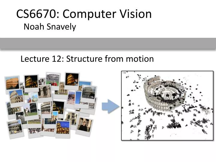
CS6670: Computer Vision. Noah Snavely. Lecture 12: Structure from motion. CS6670: Computer Vision. Noah Snavely. Lecture 13: Multi-view stereo. Announcements. Project 2 voting open later today Final project page will be released after class Project 3 out soon

E N D
CS6670: Computer Vision Noah Snavely Lecture 12: Structure from motion
CS6670: Computer Vision Noah Snavely Lecture 13: Multi-view stereo
Announcements • Project 2 voting open later today • Final project page will be released after class • Project 3 out soon • Quiz 2 on Thursday, beginning of class
Readings • Szeliski, Chapter 11.6
Fundamental matrix – calibrated case 0 { the Essential matrix
Fundamental matrix – uncalibrated case 0 the Fundamental matrix
Properties of the Fundamental Matrix • is the epipolar line associated with • is the epipolar line associated with • and • is rank 2 • How many parameters does F have? T
How many parameters? • Matrix has 9 entries • -1 due to scale invariance • -1 due to rank 2 constraint • 7 parameters in total
Stereo image rectification • reproject image planes onto a common • plane parallel to the line between optical centers • pixel motion is horizontal after this transformation • two homographies (3x3 transform), one for each input image reprojection • C. Loop and Z. Zhang. Computing Rectifying Homographies for Stereo Vision. IEEE Conf. Computer Vision and Pattern Recognition, 1999.
Rectifying homographies • Idea: compute two homographies and such that
Estimating F • If we don’t know K1, K2, R, or t, can we estimate F? • Yes, given enough correspondences
Estimating F – 8-point algorithm • The fundamental matrix F is defined by for any pair of matches p and q in two images. • Let p=(u,v,1)T and q=(u’,v’,1)T, each match gives a linear equation
8-point algorithm • In reality, instead of solving , we seek unit vector f that minimizes • least eigenvector of • need at least 8-correspondences
8-point algorithm • To enforce that F is rank 2, we replace F with F’ that minimizes subject to the rank constraint. • This is achieved by SVD. Let , where • , let • then is the solution.
8-point algorithm % Build the constraint matrix A = [x2(1,:)‘.*x1(1,:)' x2(1,:)'.*x1(2,:)' x2(1,:)' ... x2(2,:)'.*x1(1,:)' x2(2,:)'.*x1(2,:)' x2(2,:)' ... x1(1,:)' x1(2,:)' ones(npts,1) ]; [U,D,V] = svd(A); % Extract fundamental matrix from the column of V % corresponding to the smallest singular value. F = reshape(V(:,9),3,3)'; % Enforce rank2 constraint [U,D,V] = svd(F); F = U*diag([D(1,1) D(2,2) 0])*V';
8-point algorithm • Pros: • linear, easy to implement and fast • Cons: • minimizes an algebraic, rather than geometric error • susceptible to noise
! Problem with 8-point algorithm ~100 ~10000 ~100 ~10000 ~10000 ~100 ~100 1 ~10000 Orders of magnitude difference between column of data matrix least-squares yields poor results
Normalized 8-point algorithm normalized least squares yields good results Transform image to ~[-1,1]x[-1,1] (0,500) (700,500) (-1,1) (1,1) (0,0) (0,0) (700,0) (-1,-1) (1,-1)
Normalized 8-point algorithm [x1, T1] = normalise2dpts(x1); [x2, T2] = normalise2dpts(x2); A = [x2(1,:)‘.*x1(1,:)' x2(1,:)'.*x1(2,:)' x2(1,:)' ... x2(2,:)'.*x1(1,:)' x2(2,:)'.*x1(2,:)' x2(2,:)' ... x1(1,:)' x1(2,:)' ones(npts,1) ]; [U,D,V] = svd(A); F = reshape(V(:,9),3,3)'; [U,D,V] = svd(F); F = U*diag([D(1,1) D(2,2) 0])*V'; % Denormalise F = T2'*F*T1;
What about more than two views? • The geometry of three views is described by a 3 x 3 x 3 tensor called the trifocal tensor • The geometry of four views is described by a 3 x 3 x 3 x 3 tensor called the quadrifocal tensor • After this it starts to get complicated… • No known closed-form solution to the general structure from motion problem
Multi-view stereo Stereo Multi-view stereo
Point Grey’s ProFusion 25 CMU’s 3D Room Multi-view Stereo Point Grey’s Bumblebee XB3
Multi-view Stereo Input: calibrated images from several viewpoints Output: 3D object model Figures by Carlos Hernandez
Fua Seitz, Dyer Narayanan, Rander, Kanade Faugeras, Keriven 1995 1997 1998 1998 Goesele et al. Hernandez, Schmitt Pons, Keriven, Faugeras Furukawa, Ponce 2004 2005 2006 2007
error depth Stereo: basic idea
Choosing the stereo baseline What’s the optimal baseline? • Too small: large depth error • Too large: difficult search problem all of these points project to the same pair of pixels width of a pixel Large Baseline Small Baseline
z width of a pixel width of a pixel pixel matching score z
Multibaseline Stereo Basic Approach • Choose a reference view • Use your favorite stereo algorithm BUT • replace two-view SSD with SSSD over all baselines Limitations • Only gives a depth map (not an “object model”) • Won’t work for widely distributed views:
Problem: visibility • Some Solutions • Match only nearby photos [Narayanan 98] • Use NCC instead of SSD,Ignore NCC values > threshold [Hernandez & Schmitt 03]
Popular matching scores • SSD (Sum Squared Distance) • NCC (Normalized Cross Correlation) • where • what advantages might NCC have?
Known Scene Unknown Scene • Forward Visibility • known scene • Inverse Visibility • known images The visibility problem Which points are visible in which images?
Volumetric stereo Scene Volume V Input Images (Calibrated) Goal: Determine occupancy, “color” of points in V
Discrete formulation: Voxel Coloring Discretized Scene Volume Input Images (Calibrated) • Goal: Assign RGBA values to voxels in V • photo-consistent with images
True Scene All Scenes (CN3) Photo-Consistent Scenes Complexity and computability Discretized Scene Volume 3 N voxels C colors
Issues Theoretical Questions • Identify class of all photo-consistent scenes Practical Questions • How do we compute photo-consistent models?
Voxel coloring solutions • 1. C=2 (shape from silhouettes) • Volume intersection [Baumgart 1974] • For more info: Rapid octree construction from image sequences. R. Szeliski, CVGIP: Image Understanding, 58(1):23-32, July 1993. (this paper is apparently not available online) or • W. Matusik, C. Buehler, R. Raskar, L. McMillan, and S. J. Gortler, Image-Based Visual Hulls, SIGGRAPH 2000 ( pdf 1.6 MB ) • 2. C unconstrained, viewpoint constraints • Voxel coloring algorithm [Seitz & Dyer 97] • 3. General Case • Space carving [Kutulakos & Seitz 98]
Reconstruction from Silhouettes (C = 2) Binary Images • Approach: • Backproject each silhouette • Intersect backprojected volumes
Volume intersection Reconstruction Contains the True Scene • But is generally not the same • In the limit (all views) get visual hull • Complement of all lines that don’t intersect S
Voxel algorithm for volume intersection Color voxel black if on silhouette in every image • for M images, N3 voxels • Don’t have to search 2N3 possible scenes! O( ? ),
Properties of Volume Intersection Pros • Easy to implement, fast • Accelerated via octrees [Szeliski 1993] or interval techniques [Matusik 2000] Cons • No concavities • Reconstruction is not photo-consistent • Requires identification of silhouettes