Download
1 / 36
370 likes | 738 Views
Computer Vision – Compression(2). Hanyang University Jong-Il Park. Topics in this lecture. Practical techniques Lossless coding Lossy coding Optimum quantization Predictive coding Transform coding. Lossless coding. =Error-free compression =information-preserving coding General steps

E N D
Computer Vision – Compression(2) Hanyang University Jong-Il Park
Topics in this lecture • Practical techniques • Lossless coding • Lossy coding • Optimum quantization • Predictive coding • Transform coding
Lossless coding =Error-free compression =information-preserving coding • General steps • Devising an alternative representation of the image in which its interpixel redundancies are reduced • Coding the representation to eliminate coding redundancies
Huffman coding • Most popular coding (Huffman[1952]) • Two step approach • To create a series of source reduction by ordering the probabilities of the symbols and combining the lowest probability symbols into a single symbol that replaces them in the next source reduction • To code each reduced source, starting with the smallest source and working back to the original source • Instantaneous uniquely decodable block code • Optimal code for a set of symbols and probabilities subject to the constraint that the symbols be coded one at a time.
Arithmetic coding • Non-block code • One-to-one correspondence between source symbols and code words does not exist. an entire sequence of source symbols is assigned a single arithmetic code word. • As the length of the sequence increases, the resulting arithmetic code approaches the bound established by the noiseless coding theorem. • Practical limiting factors • The addition of the end-of-message indicator • The use of finite precision arithmetic
Eg. Arithmetic code 0.068
LZW coding • Lempel-Ziv-Welch coding • Assigning fixed-length code words to variable length sequences of source symbols but requires no a priori knowledge of the probability of occurrence of the symbols to be encoded • Generating a dictionary(=codebook) as the encoding proceeds. • The size of the dictionary is an important parameter. => trade-off • Applied to GIF, TIFF, PDF format and many zip algorithm
2D Run-length coding • Relative address coding(RAC)
Lossless predictive coding Principle: De-correlating data by prediction = entropy reduction
Eg. Lossless predictive coding Histogram
Lossy compression • Approaches • Predictive coding • Transform coding • Vector quantization • Etc. • Significant data reduction compared with lossless compression at the expense of quality degradation
Lossy predictive coding Prevent error accumulation
DPCM(Differential pulse code modulation) • Optimal predictor: Try to minimize the mean-square of the prediction error subject to the constraint that and
Practical prediction • Prediction for 2D Markov source • Reduction of accumulated transmission error • Typical predictors
Eg. Predictor A B C D
Optimal quantization • Minimization of the mean-square quantization error:
Lloyd-Max quantizer • Optimal quantizer in the mean-square sense • Method • Reconstruction level: centroid • Decision level: halfway • No explicit closed-form solutions for most pdfs • An iterative design procedure is applied in many cases • Optimum uniform quantizer • (uniform q.+VLC) outperforms (non-uniform q.+FLC)
Adaptive quantization • Different quantization for each subimage(eg.block) improved performance increased complexity Eg. Four different quantizers: Scaled version of the same quantizer Notice: Substantial decrease in error BUT small improvement in compression ratio
Eg. DPCM vs. Adaptive DPCM Adaptive DPCM DPCM Substantial decrease in perceived error
Transform coding • A reversible, linear transform is used • Goal: • to decorrelate the pixels of each subimage, or • to pack as much information as possible into the smallest number of transform coefficients
Comparison: Energy compaction DFT • KLT is optimal BUT it is image dependent! • DCT is a good compromise! WHT DCT Best performance
DFT vs. DCT 2n-point periodicity Less blocking artifact
Effect of subimage size • Complexity increases • Performance enhances
Eg. Block size 25% reduction Error(8x8) Org. 2x2 4x4 8x8
Bit allocation • Zonal coding • Allocation of appropriate bits for each coefficient according to the statistics • Rate-distortion theory • Eg. Gaussian pdf • Threshold coding • Global threshold • Local threshold • Fixed (N-largest coding) constant rate • Variable variable rate. Good performance
Eg. Zonal vs. Threshold Threshold better zonal
Quantization table Z • Different scaling for each coefficient. • The same quantization curve for all coefficients.
Eg. Quality control by scaling Z 34:1 67:1
Wavelet coding • New technique in 1990s • Computationally efficient • No subdivision no blocking artifact • Good performance!