Chapter 20 Model Predictive Control

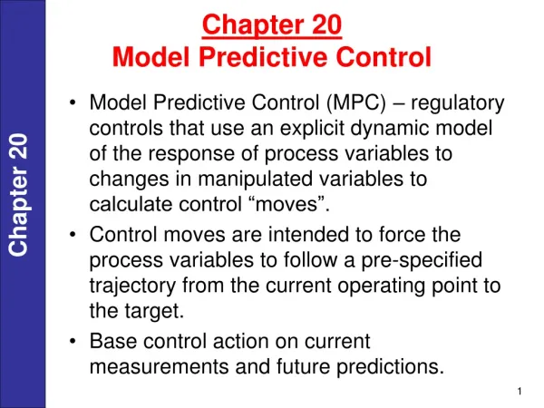
1. Chapter 20Model Predictive Control • Model Predictive Control (MPC) – regulatory controls that use an explicit dynamic model of the response of process variables to changes in manipulated variables to calculate control “moves”. • Control moves are intended to force the process variables to follow a pre-specified trajectory from the current operating point to the target. • Base control action on current measurements and future predictions.

2. Figure: Two processes exhibiting unusual dynamic behavior. (a) change in base level due to a step change in feed rate to a distillation column. (b) steam temperature change due to switching on soot blower in a boiler.

3. DMC – dynamic matrix controlbecame MPC – model predictive control • Optimal controller is based on minimizing error from set point • Basic version uses linear model, but there are many possible models • Corrections for unmeasured disturbances, model errors are included • Single step and multi-step versions • Treats multivariable control, feedforward control

4. When Should Predictive Control be Used? • Processes are difficult to control with standard PID algorithm – long time constants, substantial time delays, inverse response, etc. • There is substantial dynamic interaction among controls, i.e., more than one manipulated variable has a significant effect on an important process variable. • Constraints (limits) on process variables and manipulated variables are important for normal control.

5. Model Predictive Control Originated in 1980s • Techniques developed by industry: 1. Dynamic Matrix Control (DMC) - Shell Development Co., Cutler and Ramaker (1980), - Cutler later formed DMC, Inc. - DMC acquired by Aspentech in 1997. 2. Model Algorithmic Control (MAC) • ADERSA/GERBIOS, Richalet et al (1978) • Over 4000 applications of MPC since 1980 (Qin and Badgwell, 1998 and 2003).

6. Model Predictive Control Based on Discrete-time Models • Time-delay compensation techniques predict process output one time delay ahead. • Here we are concerned with predictive control techniques that predict the process output over a longer time horizon. (e.g., open-loop response time).

7. Figure 20.2 Basic concept for Model Predictive Control

8. General Characteristics • Targets (set points) selected by real-time optimization software based on current operating and economic conditions • Minimize square of deviations between predicted future outputs and specific reference trajectory to new targets • Discrete step response model • Framework handles multiple input, multiple output (MIMO) control problems.

9. • Can include equality and inequality constraints on controlled and manipulated variables • Solves a quadratic programming problem at each sampling instant • Disturbance is estimated by comparing the actual controlled variable with the model prediction • Usually implements the first move out of M calculated moves

10. Discrete Step Response Models Consider a single input, single output process: Where u and y are deviation variables (i.e. deviations from nominal steady-state values).

11. Discrete Convolution Models (continued) Denote the sampled values as y1, y2, y3, etc. and u1, u2, u3, etc. The incremental change in u will be denoted as Duk= uk – uk-1 The response, y(t), to a unit step change in u at t = 0 (i.e., Du0 = 1 is shown in Figure 7.14.

12. Figure 7.14 Unit Step Response

13. In Fig. 7.14, Note: hi = Si – Si-1 y1 = y0 + S1Du0 y2 = y0 + S2Du0 (Du0 = 1 for unit step . . change at t = 0) . . . . yn = y0 + SnDu0

14. Alternatively, suppose that a step change of Du1 occurred at t = Dt. Then, y2 = y0 + S1Du1 y3 = y0 + S2Du1 . . . . . . yN = y0 + SN-1Du1 If step changes in u occur at both t = 0 (Du0) and t = Dt (Du1).

15. From the Principle of Superposition for linear systems: y1 = y0 + S1Du0 y2 = y0 + S2Du0 + S1Du1 y3 = y0 + S3Du0 + S2Du1 . . . . . . yN = y0 + SNDu0 + SN-1Du1 Can extend also to MIMO Systems

16. Figure 20.8. Individual step-response models for a distillation column with three inputs and four outputs. Each model represents the step response for 120 minutes. Reference: Hokanson and Gerstle (1992).

17. Selection of Design Parameters Model predictive control techniques include a number of design parameters: N: model horizon Dt: sampling period P: prediction horizon M: control horizon (number of control moves) Q: weighting matrix for predicted errors (Q > 0) R: weighting matrix for control moves (R > 0)

18. Selection of Design Parameters (continued) 1. N and Dt These parameters should be selected so that NDt> open-loop settling time. Typical values of N: 30 <N< 120 2. Prediction Horizon, P • Increasing P results in less aggressive control action Set P = N + M • Control Horizon, M • Increasing M makes the controller more aggressive and increases computational effort, typically 5 <M< 20 • Weighting matrices Q and R • Diagonal matrices with largest elements corresponding to most important variables