Download

1 / 36
360 likes | 372 Views
Climate Extremes The Drought Hazard Bradfield Lyon International Research Institute for Climate and Society The Earth Institute, Columbia University US CLIVAR Summit on Climate Extremes Denver, CO 7-9 July 2010. US CLIVAR Drought Working Group. Drought in Coupled Models Project – “DRICOMP”.

E N D
Climate Extremes The Drought Hazard Bradfield Lyon International Research Institute for Climate and Society The Earth Institute, Columbia University US CLIVAR Summit on Climate Extremes Denver, CO 7-9 July 2010
US CLIVAR Drought Working Group Drought in Coupled Models Project – “DRICOMP”
Drought – An Extreme Challenge • Difficult to define. Fundamentally, an insufficient supply of water to meet demand • but demands are many, vary with region and sector, and supply can be of • non-local origin (e.g., Tucson, AZ and the CO River) • When does “drought” start? Terminate? As measured by what? Relevant to? • Occurs on multiple timescales – often simultaneously (consider its impacts) • In all cases, ultimately tied to “extended” periods of deficient precipitation relative • to the “expected” value for a particular location but that includes: • - Late onset or early demise of monsoon rainfall • - Monsoon breaks • - Sub-seasonal SI multi-year multi-decadal CC • Multiple causes. Linked to regional and large scale atmospheric circulation • anomalies (some related to SSTs) and land surface-atmosphere interactions • Enhanced drought prediction depends fundamentally on improved predictions • of precipitation (and other variables related to surface fluxes of water and energy)
Monitoring Drought – What Aspect? Figure: UN World Water Development Report-2, Chapter 4, Part 1. Global Hydrology and Water Resources
Monitoring Drought – Characteristic Time Scales Correlation Top Layer VIC Soil Moisture and SPI-3 (1950-2000) All Months May-Sep only Hudson Valley NY Std. VIC SM1 Anomalies (monthly, 5-yr) VIC data Courtesy of Justin Sheffield, Princeton Univ.
Monitoring Drought Numerous “drought” indices in use each with its own “intrinsic” time scale - PRCP -- monthly, past 90 days, water year, standardized indices (SPI) - Water balance indices: “P-E”, PDSI, etc. - Soil Moisture (typically modeled, experimental satellite products) - Snow Water Equivalent, Surface Water Supply Index - Streamflow - Vegetation Condition (satellite estimates) … Challenges: - Observational data are imperfect; scale issues (information, decisions) - Lack of real time updates for monitoring and prediction (“preliminary”) - Lack of long historical records for satellite-derived (and other) products - Higher frequency (daily) precipitation also of interest but often unavailable - Derived quantities (e.g. model soil moisture) subject to input uncertainties and observations for calibration/comparison are sparse - Relevance of indices (and predictions) to specific applications -- the “best” drought index is the one most closely associated with the specific application of interest (ag, rangeland condition, streamflow, etc.)
RMS Difference in Monthly PRCP GPCC – UEA as a Fraction of GPCC Annual Mean (1971-2000) To = e-folding time for run durations in SPI-12 CPC SPI-12 > +1.0 CPC SPI-12 < -1.0 e-folding time (months)
Modeled Soil Moisture Estimates (Runoff, ET, Soil Saturation) • Derived variables influenced by • uncertainties in model inputs and • different model designs • Use model-relative measures of • variability (e.g., percentiles) for • comparisons across models in • near real time • Need for enhanced observations • of soil moisture • Better flux measurements for • comparison with models (Ameriflux) Slide Courtesy of Kingtse Mo CPC Drought Briefing for May 2010
Estimates of “Soil Moisture” from Satellite SMOS – ESA; SMAP – NASA SMOS Figure: ESA
Prolonged Drought -- The Role of SSTs Schubert et al., 2004
Prolonged Drought – The Role of SSTs POGA-ML (similar to GOGA) Seager et al., 2005
Prolonged Drought – “ENSO +” Protracted Drought 1998-2002 Hoerling and Kumar, 2002
Trends: Coupled Models vs. AMIP Shin and Sardeshmukh, 2010
1988 Drought AMJ SST Anomaly AMJ PRCP & 250 hPa Std. Hght. Anomalies
AMJ 1988 Anomalous Stationary Waves Reanalysis ECHAM4.5 CFS
Observations & AMIP Simulations: Drought of 1988 SPI-6 OBS Jun 1988 SPI-6 NSIPP Jun 1988 SPI-6 ECHAM4.5 Jun 1988 SPI-6 GFDL 2.14 Jun 1988
Role of the Land Surface • GLACE-2 (GEWEX, CLIVAR) • Used best estimate of soil moisture from offline (similar to GSWP-2) • Compared control with initialized land sfc. runs across multiple GCMS (10) Koster et al., 2010
Role of the Land Surface Koster et al., 2010
Role of the Land Surface – Model Biases (GLACE) • Overall (global scale) soil moisture memory reasonably simulated • Regional biases important for the practical application of model output Seneviratne et al., 2006
Towards Probabilistic Prediction of Meteorological Drought • Predictive information from both persistence • and GCM • AMIP -- Does not include the role of land • surface condition
Observed yield (kg ha-1) Observed soybean yields (GA, USA yield trials) vs. seasonal rainfall, temperature, simulated yields Rainfall (mm day-1) Mean max temperature (°C) Simulated yield (kg ha-1) Importance of the Sub-seasonal Time Scale:Dynamic Crop Models • Account for dynamic, nonlinear crop-soil-weather interactions • Need DAILY weather inputs in crop models • Requires disaggregation of seasonal forecasts to obtain daily sequences of T, P Slide Courtesy of James Hansen, IRI
Bias-Corrected Daily Rainfall from a GCM Raw GCM Daily Rainfall: Amplitude, Frequency Bias Observed Rainfall Bias-Corrected GCM: (Amplitude, Frequency) • GCM over-estimates the OBS • autocorrelation of daily PRCP • Changes in higher-frequency • precipitation events of much • interest to ag. and water sectors • (including under CC) Ines and Hansen (2006), Hansen et al. (2006)
Demand to Move Beyond One’s Means Annual DJF JJA Figure 11.12, IPCC AR4
“Near-Normal” Monthly Precipitation in Central Park (within +/- 5% of long term median value) Cum. Days in Category No. Days with Precipitation
FIG. 2. Scatterplot of the percentage change in global-mean column-integrated (a),(c) water vapor and (b),(d) precipitation vs the global-mean change in surface air temperature for the PCMDI AR4 models under the (a),(b) Special Report on Emissions Scenarios (SRES) A1B forcing scenario and (c),(d) 20C3M forcing scenario. The changes are computed as differences between the first 20 yr and last 20 yr of the twenty-first (SRES A1B) and twentieth (20C3M) centuries. Solid lines depict the rate of increase in column-integrated water vapor (7.5% K-1). The dashed line in (d) depicts the linear fit of P to T, which increases at a rate of 2.2% K-1.
Graphic: Third UN Water Development Report, World Water Assessment Report, 2009
http://upload.wikimedia.org/wikipedia/commons/f/f2/World_population_growth_%28lin-log_scale%29.pnghttp://upload.wikimedia.org/wikipedia/commons/f/f2/World_population_growth_%28lin-log_scale%29.png
Graphic from -- Groundwater: A global assessment of scale and significance, IWMI, 2007
FIG. 2. Scatterplot of the percentage change in global-mean column-integrated (a),(c) water vapor and (b),(d) precipitation vs the global-mean change in surface air temperature for the PCMDI AR4 models under the (a),(b) Special Report on Emissions Scenarios (SRES) A1B forcing scenario and (c),(d) 20C3M forcing scenario. The changes are computed as differences between the first 20 yr and last 20 yr of the twenty-first (SRES A1B) and twentieth (20C3M) centuries. Solid lines depict the rate of increase in column-integrated water vapor (7.5% K-1). The dashed line in (d) depicts the linear fit of P to T, which increases at a rate of 2.2% K-1.
US CLIVAR DWG -- Idealized SST Runs Drought Working Group • Work done in parallel with the • Drought in Coupled Models • Project (DRICOMP)