Download
1 / 61
610 likes | 824 Views
Inventory Systems for Independent Demand. OPERATIONS MANAGEMENT CLASS. This presentation explores: The definition and purpose of inventory Inventory costs Independent vs. dependent demand Basic fixed order quantity system Basic fixed time period system

E N D
Inventory Systems for Independent Demand OPERATIONS MANAGEMENT CLASS • This presentation explores: • The definition and purpose of inventory • Inventory costs • Independent vs. dependent demand • Basic fixed order quantity system • Basic fixed time period system • Customer Service - Achieving Percent Fill Rates
Inventory • Definition--The stock of any item or resource used in an organization • Raw materials • Finished products • Component parts • Supplies • Work in process ....
INV. MANAGEMENT OBJECTIVES • MAXIMUM CUSTOMER SERVICE • MINIMUM INV. INVESTMENT • MAXIMUM EFFICIENCY (MIN. COST) • MAXIMUM PROFIT • HIGHEST RETURN ON INVESTMENT • TO USE INVENTORY FOR STRATEGIC ADVANTAGE
TRADE-OFFS • YOU CAN’T SELL FROM AN EMPTY CART • OUR LINE OF CREDIT (BUDGET) WILL SUPPORT ONLY SO MUCH • $1 IN INVENTORY COSTS ABOUT $.25/YEAR • OUT-OF-STOCKS > LOST SALES > LOST CUSTOMERS • OUR SHAREHOLDERS WANT A 15% ROI • ITS IMPOSSIBLE TO FORECAST PERFECTLY
Purposes of Inventory 1. To maintain independence of operations 2. To meet variation in product demand 3. To allow flexibility in production scheduling 4. To provide a safeguard for variation in raw material delivery time 5. To take advantage of economic purchase-order size TO DECOUPLE AND ECONOMIC LOT SIZE.
3 QUESTIONS OF INVENTORY SYSTEM • WHAT TO ORDER? • HOW MANY TO ORDER? • WHEN TO ORDER? • TIMING IS A CRITICAL ISSUE!
Inventory Costs • Holding (or carrying) costs • Setup (or production change) costs • Ordering costs • Shortage costs ....
SEVERAL DIFFERENT SYSTEMS • INDEPENDENT DEMAND - MUST BE FORECASTED. • WAGONS, BICYCLES, ETC. • FINISHED GOODS OR SERVICES • DEPENDENT DEMAND - CAN AND SHOULD BE CALCULATED • WHEELS, SPOKES, HANDLE BARS • COMPONENTS FOR SERVICES • SIMPLE BUT POWERFUL PRINCIPLE
Independent vs. Dependent Demand Independent Demand (Demand not related to other items) Dependent Demand (Derived) E(1) ....
Classifying Independent Demand Systems • Fixed-Order Quantity • Fixed-Time Period • Hybrid Systems - Both Together - Order Periodically unless we reach the reorder point.
Fixed-Order Quantity Models Idle state Waiting for demand Demand occurs Unit withdrawn from inventory or back ordered No Is status < Reorder point? Compute inventory status Status = On hand + On order - Back order Yes Issue order for Exactly Q units ....
Fixed-Order Quantity ModelsAssumptions • Demand for the product is constant and uniform throughout the period • Lead time (time from ordering to receipt) is constant • Price per unit of product is constant ....
Fixed-Order Quantity ModelsAssumptions • Inventory holding cost is based on average inventory. • Ordering or setup costs are constant. • All demands for the product will be satisfied (No back orders are allowed) ....
Q Q Q R L L Time EOQ Model--Basic Fixed-Order Quantity Model Number of units on hand R = Reorder point = L*d Q = Economic order quantity L = Lead time d = Demand per Unit of Time ....
Cost Minimization Goal TAHC = H*(Q/2) TAOC = S*D/Q TAC = TAHC + TAOC C O S T Total Cost Holding Costs Annual Cost of Items (DC) Annual Ordering Costs QOPT Order Quantity (Q) ....
Annual Purchase Cost Total Annual Ordering Cost Total Annual Holding Cost Total Annual Cost = + + Basic Fixed-Order Quantity Model TC Total annual cost D Demand C Cost per unit Q Order quantity S Cost of placing an order or setup cost R Reorder point L Lead time H Annual holding and storage cost per unit of inventory ....
Deriving the EOQ - Calculus Method • Using calculus, we take the derivative of the total cost function and set the derivative (slope) equal to zero ....
Deriving the EOQ - Graphical Method • Recognizing TAHC = TAOC at Optimal • TAHC = H*Q/2 TAOC = S*D/Q • H*Q/2 = S*D/Q, Solving for Q Yields:
EOQ Example Annual Demand = 1,000 units Days per year considered in average daily demand = 365 Cost to place an order = $10 Holding cost per unit per year = $2.50 Lead time = 7 days Cost per unit = $15 Determine the economic order quantity and the reorder point. ....
Solution Why do we round up? ....
In-Class Exercise Annual Demand = 10,000 units Days per year considered in average daily demand = 365 Cost to place an order = $10 Holding cost per unit per year = 10% of cost per unit Lead time = 10 days Cost per unit = $15 Determine the economic order quantity and the reorder point. Note: (Tag hidden-slide icon to project solution) ....
ACHIEVING HIGH CUSTOMER SERVICE • ADD BUFFER STOCK • ORDER EARLIER • ACHIEVE DESIRED CUSTOMER SERVICE • PERCENT FILL RATE = .99 = 9,900/10,000 ARE SUPPLIED DIRECTLY FROM STOCK
Q Q Q R = dL + B = dL + ZSL L L Time ADDING SAFETY STOCK TO ORDER EARLIER • Fixed Order Quantity System Under Uncertainty B = ADD BUFFER STOCK IN CASE DEMAND DURING LEADTIME > EXPECTED, d*L. R = Reorder point Q = Economic order quantity L = Lead time SL = Standard Error of Estimate During Leadtime B = Buffer stock set to achieve P
STRATEGIC IMPORTANCE OF %FILL (P) • P IS SET BY TOP MANAGEMENT • P IS STRATEGIC PERFORMANCE MEASURE • CONTEMPORARY P ARE INCREASING • P=99.8 IS BECOMING MORE COMMON • HOW DO WE CONTROL INVENTORIES TO ACHIEVE P?
THE VARIANCE LAW IF X AND Y ARE INDEPENDENT RANDOM VARIABLES AND Z = X + Y THEN __ __ __ Z = = X + Y AND Z2 = X2 + Y2 ______________ Z = X2 + Y2 This is extremely important in many applications.
EXAMPLES OF THE VARIANCE LAW CPM – with Critical Path Consisting of activities A, C, D, F, and G Tcp = TA + TC + TD + TF + TG = Mean time of CP AND CP2= A2 + C2 + D2 + F2 + G2= Var of CP ______________ This is extremely important in many applications. For example if A, C, D, F, and G were stock returns from investments then the average returns and variances equal those of the above assuming they are independent of each other. In forecasting/inventory control we see that:
FORECASTING DEMAND DURING LT • MEAN DEMAND = d*L • Where L is length of LT • Assume L = 3, d = SEE in forecasting, • L = SEE during leadtime. ___ • L = d1 +d2 + d3 = d L • This Assumes Demand is Normally Independently Distributed • This Allows the Use of the E(Z) Concept
STATISTICAL INVENTORY CONTROLSCIENTIFIC INVENTORY CONTROL • SCIENTIFICALLY SET THE REORDER POINT TO YIELD DESIRED PERCENT FILL (P) • R= dL + ZL = Mean + Buffer Stock where • R = Reorder Point • dL = Mean Demand During Leadtime • L = Standard Error of Forecast During LT • Z = Value Determined to Achieve P
DETERMINING THE BEST Z-VALUE • (1-P)D = No. Units Short Per Year • E(Z) = Units Short Per Leadtime when L is 1. • No. Units Short Per Year = E(Z)* L*D/Q • Equating Both • E(Z)* L*D/Q = (1-P)D rearranging: • E(Z) = (1-P)Q/ L
E(Z) = (1-P)Q/ L • THIS RELATES THE FOLLOWING: • PERCENT FILL RATE (P) • FORECAST ACCURACY • SAFETY STOCK • ORDER QUANTITY • NO. OF EXPOSURES PER YEAR • REORDER POINT
LET’S WORK A PROBLEM • D=5000, P=.99, C=$3/UNIT, i=.20$/$/YR • S=$10, d=100, d=30, L=3 • Determine the EOQ • Reorder Point • Safety Stock • Annual Investment in Inventory • Comment on the effectiveness of this solution.
Compute inventory status Status = On hand + On order - Back order Compute order quantity to bring inventory up to required level Issue an order for the number of units needed Fixed-Time Period Model No Is it Time to Place an Order? Yes Idle state Waiting for demand Demand occurs Unit withdrawn from inventory or back ordered ....
d*T L L Time Fixed-Time Period System Under Certainty q = d*(T+L) - I - On Order_____ ______________________ Number of units on hand d*T d*T T <----------T--------> <-------T------------> Average Q = d*T T = Time between review L = Lead time d = Demand per Unit of Time ....
d*T L L Time Fixed-Time Period System - Under Uncertainty q = d*(T+L) + Buffer Stock - I - On Order____________ Number of units on hand d*T d*T T <---------T---------> <-------T------------> Average Q = d*T T = Time between review L = Lead time d = Demand per Unit of Time ....
FORECASTING DEMAND DURING L+ T PERIODS • MEAN DEMAND = d*L • _____ • STD. DEV. L+T = d T + L • We Assume Demand is Normally Distributed • This Allows the Use of the E(Z) Concept
Determining the Value of T+L • The standard deviation of a sequence of random events equals the square root of the sum of the variances ....
Example--Fixed-Time Period Model Daily demand for a product is 20 units. The review period is 30 days, and lead time is 10 days. Management has set a policy of satisfying 96 percent of demand from items in stock. At the beginning of the review period there are 200 units in inventory. The daily demand standard deviation is 4 units. How many units should be ordered? ....
Solution No Interpolation, always choose the Highest Z value E(Z) Z 1.00 -0.90 0.92 -0.80 ....
Solution (continued) To satisfy 96 percent of demand order 580 units at this review period. ....
Compute inventory status Status = On hand + On order - Back order Compute order quantity to bring inventory up to required level Issue an order for the number of units needed Hybrid Model - Fixed-Time Period Model No Time to Place an Order or is status < Reorder point? Yes Idle state Waiting for demand Demand occurs Unit withdrawn from inventory or back ordered ....
Miscellaneous SystemsOptional Replenishment System Maximum Inventory Level, M q = M - I Actual Inventory Level, I M I Q = minimum acceptable order quantity If q > Q, order q. ....
Miscellaneous SystemsBin Systems Two-Bin System Order One Bin of Inventory Full Empty One-Bin System Order Enough to Refill Bin Periodic Check ....
60 % of $ Value A 30 B C 0 % of Use 30 60 ABC Classification System • Items kept in inventory are not of equal importance in terms of: • dollars invested • profit potential • sales or usage volume • stock-out penalties ....
VILFREDO PARETO • FAMOUS ITALIAN MATH., ECON. AND ENGI. • SMALL % OF POP GET LARGE % OF INCOME • 20-80 RULE (SMALL/LARGE) • 80% OF SALES FROM 20% PRODUCTS • 80% OF PROFITS FROM 20% OF PRODUCT • 80% SALES FROM 20% OF PEOPLE • 95% OF PROBLEMS FROM 5% OF CAUSES • OTHER EXAMPLES
ALLOCATE CONTROL RESOURCES TO THE VITAL FEW • CONSIDER ANNUAL DOLLAR USAGE • HIGHEST ANNUAL USAGE ARE “A” ITEMS • REMAINING ARE “B” AND “C” ITEMS • MORE CLOSELY CONTROL “A” • LESS CLOSELY CONTROL “B” AND “C” • ASSURE THAT WE DO NOT RUN OUT OF STOCK OF ANY ITEMS • CONSIDER AN EXAMPLE
CONSIDER A PURCHASING DEP’T • 30 ORDERS PER YEAR IS MAX. ACTIVITY • 80 MIL OF A ITEMS • 15 MIL OF B ITEMS • 5 MIL OF C ITEMS • EACH ARE ORDERED 10 TIMES PER YEAR
ITEM $ # Q Q/2 H*Q/2 • A 80 10 8 4 .25*4 = 1.000 • B 15 10 1.5 .75 .1875 • C 5 10 .5 .25 .0625 • 5.0 1.25 • A 80 20 4 2 .5 • B 15 5 3 1.5 .375 • C 5 5 1 .5 .125 • 4.0 1.00
Inventory Accuracy and Cycle Counting • Inventory accuracy - Bank Teller Vs. Store Room • Do inventory records agree with physical count? • Eliminate the Causes of Errors • Eliminate the Errors • Cycle Counting • Frequent counts • Which items? • When? • By whom?