Download
1 / 19
190 likes | 279 Views
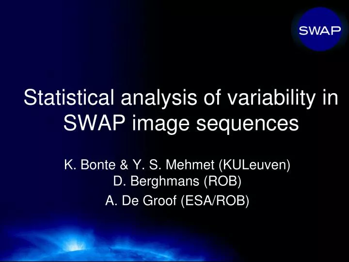
Statistical analysis of variability in SWAP image sequences. K. Bonte & Y. S. Mehmet (KULeuven) D. Berghmans (ROB) A. De Groof (ESA/ROB). Understanding SWAP variability. Sequence of 1024x1024 PIXELS. APS: Every pixel has its own personality!

E N D
Statistical analysis of variability in SWAP image sequences K. Bonte & Y. S. Mehmet (KULeuven)D. Berghmans (ROB) A. De Groof (ESA/ROB)
Understanding SWAP variability Sequence of 1024x1024 PIXELS • APS: Every pixel has its own personality! • How do we distinguish between instrumental variability and solar variability? • Knowing each pixel’s behavior, how do averages over subfields behave? • How do we know in which subfield of SWAP the flare happens? • How does the SWAP total intensity timeline relate to LYRA, GOES curves? katrien subfields Sarp 1 timeline
SWAP AVERAGE INTENSITY OVERALL TREND (April 1st-May 21st)
SWAP average intensity ON 2010/05/08 LARGE ANGLE ROTATIONS (LARs) - Downward spikes correspond to LARs - LAR Periodicity ~24.5 min
SWAVINT ON 2010/05/08 SOUTH ATLANTIC ANOMALY * -> South Atlantic Anomaly
SWAVINT ON 2010/05/08 C 9.3 FLARE (GOES peak 07:42) C9.3 flare
SWAVINT ON TUESDAY 2010/05/11 LED IMAGES
SWAVINT ON 2010/05/19 OFF-POINTING
SWAP average intensity (SWAVINT keyword) Background EUV trend well recovered. SWAP can be used as a radiometer: 5th LYRA channel individual flares hardly observable. Big flares TBC. Subfields? signal dominated by spacecraft rolls, SAA, instrument off-pointing and LEDS.
Statistical analysis of variability in SWAP image-sequences: Local variability K.Bonte – Centre for Plasma Astrophysics
Why local variability? • Swap_average gives an idea of overall variability(similar to Lyra data but for narrow bandpass, centered around 17.5 nm) • We want to zoom into regions of interest, locate intresting subfields • Active Regions • Events • Flares (possibly working towards flare-detection) • … • Get an idea of how active a located Active Region really is.. K.Bonte – Centre for Plasma Astrophysics
First step • Look at variability of intensity in time, at pixel-level. • Differentiate “instrumental noise” from variability in intensity due to solar activity. • INPUT: time-sequence of SWAP images Int. • OUTPUT, PER PIXEL (over time sequence): • - average intensity <Intpixel> • - standard deviation <Ip> + <Intpixel> <Ip> - Time K.Bonte – Centre for Plasma Astrophysics
An example: Sequence of 64 dark images (off limb,10sec). a) Median st.dev. b) Logscaledmedian st.dev. • This result tells us: • (b) Estimate for the dark noise by extrapolating the result for <Int>=0 +- pre-launch calibration value: 1,9 DN. • (a) Each point corresponds to (average intensity, st.dev.) of 1 pixel. Each average intensity value ~ different values of st.dev. per pixel. Because CMOS ≠ CCD!!Every pixel of a CCD detector would show +- the same behaviour (~PTC).SWAP uses a CMOS detector.. <Intpixel> <Intpixel>
CMOS ≠ CCD customized PTC • CCD detector ~ Photon Transfer Curve =expected noise as function of intensity,for each pixel the same. - Readout_noise: slope=0 - Photon Shot Noise: slope=0,5 - Fixed Pattern Noise: slope=1 • CMOS detector: Every pixel suffers extra instrumental noise due to extra electronics per pixel. • To differentiate instrumental noise: need to understand behaviour of each pixel. • First challenge: provide a “customized Photon Transfer Curve” per pixel! <Intpixel>
Customized PTC per pixel • Working on pixel-level, results in 1 value (1point) per image-sequencein the [<Int> - st.deviation] diagram. • We aim to fit a polynomial function through points that we retrieve from darks + led data (different sequences), simulating intensities from dark currents up to solar intensity. Function based on PTC: <Intpixel> 2 (x,y) = dark_noise + (x,y)*Int(x,y) + (x,y)*Int 2(x,y) slope=0 + slope=0,5 + slope=1 cte + PSN + FPN relating a value of “instrumental noise” to average intensity, per pixel.
Application • Differentiate “instrumental noise” from intensity variability due to solar activity. • In histograms of standard deviation PER PIXEL (or group of pixels): signal <--> instrumental Intresting subfield Less intresting subfield K.Bonte – Centre for Plasma Astrophysics
Application • Differentiate instrumental noise from intensity variability due to solar activity. • In time-intensity plots PER PIXEL (or group of pixels): Comparing per pixel peaks of intensity with instrumental noise of that pixel (value from customized PTC): locating intresting subfields <Intpixel> +3* <Intpixel>
To be continued... Thanks K.Bonte – Centre for Plasma Astrophysics