Download
1 / 60
610 likes | 953 Views
ACA 2014 Applications of Computer Algebra Session: Integration: implementation and applications Fordham University New York, NY, USA, July 9-12. Piecewise Functions and Convolution Integrals. Michel Beaudin, Frédérick Henri, ÉTS , Montréal, Canada. Introduction

E N D
ACA 2014 Applications of Computer Algebra Session: Integration: implementation and applications FordhamUniversity New York, NY, USA, July 9-12 Piecewise Functions and Convolution Integrals Michel Beaudin, Frédérick Henri, ÉTS, Montréal, Canada
Introduction • Convolution of two functions : • Case of Laplace transforms • Continuous LTI systems • Computing the convolution • Symbolic Convolution in Nspire CAS • Conclusion • Overview
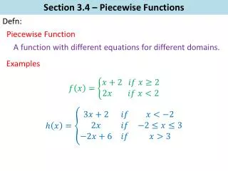
Why this subject? At the last ACA conference, we showed how useful it was for a Computer Algebra System (CAS) to perform symbolic integration of Piecewise Continuous Functions (PCF) and expressions containing such functions. Sadly, Texas Instruments computer algebra system Nspire CAS is able to deal with PCF but presents some limitations. Introduction
Let a PCF be defined over an interval (or the entire real line) and be continuous over each sub-interval. Here is what Nspire CAS does well : • The symbolic derivative, the symbolic indefinite integral and the symbolic definite integral. • The system correctly checks the endpoints for the derivative and adjusts the constants of integration for each sub-interval for the integral. • Introduction
Here is an example. Introduction Constants are addedto obtain a continuous antiderivative. Exact value.
Function f(x) and definite integral: Introduction
Important: a continuous antiderivative! Introduction
We just saw that Nspire CAS uses templates to define piecewise functions. These templates are attractive but some limitations appear if one wants to perform more complicated symbolic operations. Introduction
As an example, we continue with our earlier function y = f(x) and try to compute . Introduction Unable to compute! No exact value!
Nspire CAS built-in integrator is unable to perform the symbolic integration of a product of a single expression with a piecewise function. Furthermore, it only returns a floating point approximation for the definite integral. Introduction
This is why Frédérick Henri has programmed some functions (showed last year at ACA). With these functions (included in a special library used by us at ETS), Nspire CAS is now able to do all of this correctly! Introduction
Here is a brief recap of how it works: • We group into a single piecewise function an expression using the function grouper_fct(ex, var) where ex is an expression in variable var. • Introduction
We use the built-in integrator of Nspire CAS to perform the integral. Note that in the upcoming slide: • kit_ETS_fh\integral_mcx(ex, var) stands for the indefinite integral of exwrt to var. • kit_ETS_fh\integral_mcx_d(ex, var, lo, up) stands for the definite integral of exwrtvar from lo to up. • Introduction
Introduction Nspire CAS built-in integrator. Only a floating point approximation. Symbolicpiecewiseantiderative! Exact value!
Case of Laplace transforms Usually, students are introduced to Laplace transforms inside an ODE course. Functions f(t) are defined for and the Laplace transform of f is the function F defined by the improper integral Convolution of Two Functions
Case of Laplace transforms Let’s use the notation for the correspondence between the function f(t) and its transform F(s). Note that f(t) is in fact f(t) u(t) where u(t) is the unit-step function (Heaviside function): Convolution of Two Functions
Case of Laplace transforms Then we have the “convolution property” This last integral is called the convolution (in the sense of Laplace transforms) of f and g. Convolution of Two Functions
Case of Laplace transforms Note that it can be written in the more general form if x(t) = f(t)u(t) and h(t) = g(t)u(t). Convolution of Two Functions
Case of Laplace transforms Unfortunately, in a classical ODE course, few words are said about convolution or the reasons why it is important. For simplicity, let’s take a linear second order, constant coefficients ODE Convolution of Two Functions
Case of Laplace transforms Then the solution of is given by the convolution where h(t) is known as the impulse response and H(s) as the transfer function. Convolution of Two Functions
Case of Laplace transforms Usually, the ODE represents a damped mass-spring problem or a RLC circuit problem. In this case, the coefficients a, b and c are positive and there is no loss of generality taking zero initial conditions since the transient solution dies out. So, the convolution solves the ODE. Convolution of Two Functions
Continuous LTI systems We now consider a (continuous) system where an input x(t) enters the system and an output y(t) is produced. Some examples: Convolution of Two Functions x(t) SYSTEM y(t)
Continuous LTI systems Another example is a mass-spring system: the external force f(t) is the input (f(t) = 0 if t < 0) and the position y(t) of the object at time t is the output. The following ODE is the model used: Convolution of Two Functions Constant of friction Mass of the object Spring constant
Continuous LTI systems Let the input produce the output and let the input produce the output . The system is linear if the linearly combined input produces the linear combined output Convolution of Two Functions
Continuous LTI systems Let the input x(t) produces the output y(t), let a be any real number. The system is time-invariant if the shifted output y(t - a) is the same as the output produced by the shifted input x(t - a). That is: S(x(t)) = y(t) S(x(t - a)) = y(t - a) Convolution of Two Functions
Continuous LTI systems The system is said linear, time-invariant (LTI) if both conditions are satisfied. Example: consider again the capacitor as a system. When a current i(t) passes through the capacitor C, the voltage across the capacitor is Convolution of Two Functions
Continuous LTI systems This is a linear system because of the linearity of the integral. The system is also time-invariant as a change of variable shows it. Convolution of Two Functions
Computing the convolution In signal analysis courses, students learn how to compute by hand the convolution of two signals. They are introduced to important functions such as unit step function u(t) and unit-impulse (Dirac delta) “function” d(t). But there is no need to deal with the theory of generalized functions. Convolution of Two Functions
Computing the convolution Instead, they are using limiting process. The Dirac delta “function” is replaced by an approximate unit-impulse function: In Derive, this is nothing else than Convolution of Two Functions
Computing the convolution Given a system, the output to the unit-impulse d(t) is called the system impulse responseh(t). Fact: in a continuous LTI system, the output y(t) to the input x(t) is given by the convolution Convolution of Two Functions
Computing the convolution This is easy to justify. The signal x(t) is replaced by a staircase approximation and a limit: If is the output to , then the linearity of the integral and time invariance yields the result. Convolution of Two Functions
Computing the convolution Suppose you want to perform a convolution: Then, 4 steps must be completed : reverse the time in the signal h; shift the variable; multiply by the signal x; integrate over all values of t, doing this for every value of t. Convolution of Two Functions
Computing the convolution For example, the convolution of two rectangular pulses of finite (but different) duration is a trapezoidal signal: Let’s switch to Nspire CAS and show an animation of this. Convolution of Two Functions Convolution of x(t) and h(t).
Computing the convolution Derive can easily perform the last convolution because of its ability to integrate piecewise functions. Even though the Dirac delta function has never been implemented into Derive, we can compute symbolic limits involving indicator functions. So we can use impulse functions! Convolution of Two Functions
Computing the convolution Let us show a Derive screen where the convolution is defined. Then we will show the convolution of the two rectangular pulses x(t) = CHI(0, t, 1) and h(t) = 1.5CHI(0, t, 2). In Derive, CHI(a, x, b) is the indicator function of the open interval a< x < b. The notation is c(a, x, b). Convolution of Two Functions
Computing the convolution Finally, we will illustrate the fact that the convolution with the shifted Dirac delta function d(t - a) produces a translation on a signal x(t): The next slide shows this with a = 1. Convolution of Two Functions
Convolution of Two Functions It issoeasy to definea convolution of 2 signalsin Derive! Wetake 2 rectangular pulses, usingthe indicatorfunctionc of Derive. Hereis the result and the graph. Nowweconvolvethe « output » withd(t- 1), usinga limit of indicatorfunction: thisproduces, as expected, a translation of the signal « output ».
We know Nspire CAS can’t simplify the product of a piecewise expression with another expression. So, if x(t)is piecewise with compact support, the integral of x(t) with another expression only yields a floating point value. The next slide illustrates this. Symbolic Convolution in Nspire CAS
Here is, again, an example. Now let’s try to perform the convolution of x(t) and h(t). Symbolic Convolution in Nspire CAS No exact value. Exact value!
Nspire CAS built-in integrator won’t succeed … Symbolic Convolution in Nspire CAS Oups…!
… neither will Frédérick’s function! Symbolic Convolution in Nspire CAS
So, what can we do? Our goal is to find a way for Nspire CAS to compute the symbolic convolution without giving up the use of templates. As far as integration is concerned, endpoints of each subinterval are irrelevant. Symbolic Convolution in Nspire CAS
Here is what we will do: • Convert a piecewise function into a linear combination of signum functions. • Import from Derive a very important rule: • Symbolic Convolution in Nspire CAS
Perform the symbolic integration of each term. • Convert the result into a piecewise expression (if applicable). • Moreover, if one needs to use a Dirac delta function, it should be possible to achieve, using limit of indicator functions. • Symbolic Convolution in Nspire CAS
Note : the rule yields a continuousantiderivative. Here is why. Let G(x) be an antiderivative of F(x). Consider the function “Albert”: This function is everywhere continuous and differentiable except at the point x = -b/a. Symbolic Convolution in Nspire CAS
The derivative of SIGN(ax + b) is 0 except at x = -b/a. So, for x ≠ -b/a, For x ≠ -b/a, Albert(x) is continuous everywhere because SIGN and G are continuous. If x= -b/a, it is also continuous because SIGN is a bounded function: Symbolic Convolution in Nspire CAS
New functions were defined and saved in an updated version of the library Kit_ETS_FH. Frédérick Henri took care of the programming side of the job and Michel Beaudin took care of the mathematical requests. Here is a description of the principal functions. Symbolic Convolution in Nspire CAS
The sign function is already implemented into Nspire CAS. We have defined the unit step function and the piecewise indicator function of the interval ]a, b[: Frédérick’s function unpiece transforms a piecewise function into a linear combination of indicator functions. The inverse is achieved with the function signtopiece. Symbolic Convolution in Nspire CAS
Here are some examples: Symbolic Convolution in Nspire CAS Weadd the « step » function. Weadd the indicatorfunction and call it « chi ». We « unpiece ». We« convert » to piecewise. « grouper_fct » finishes the job.
Nspire CAS is now able to do as Derive when comes time to integrate a product of sign with another expression. In fact, Frédérick has programmed the function integral_sign in order to compute the integral of expressions as sign(ax + b)·f(x). For more complicated examples, expansion is used and the function integral2 does the job. Let’s take a look at an example. Symbolic Convolution in Nspire CAS