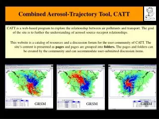
Combined Aerosol Trajectory Tool, CATT Illustrated Instruction Manual

1. Combined Aerosol Trajectory Tool, CATTIllustrated Instruction Manual Supported by: MARAMA contract on behalf of Mid-Atlantic/Northeast Visibility Union (MANE-VU) for theInter-RPO Workgroup for Data Analysis Supplemental funding from Environmental Protection Agency, OAQPS , Agreement # 83114101-0 National Science Foundation, Grant #0113868 Performed by the Center for Air Pollution Impact and Trend Analysis (CAPITA, Washington University In collaboration with Cooperative Institute for Research in the Atmosphere, CIRA-VIEWS Program January 10, 2004

2. Acknowledgements • The CATT Tool is the result of an effective CIRA-CAPITA collaboration to create a sequential value-adding chain. CIRA has opened the VIEWS and the ATAD databases for use by CAPITA. In fact the current CATT ensemble trajectory browser is accessing the VIEWS database for chemical data in real time! CAPITA added the trajectory browser code and the user interface. • The result is a textbook illustration of the new distributed computing paradigm! It is hoped that the values that the CATT project added to the chain will be accessed and utilized by others and continue the value-adding process. The opportunities for mutual empowerment are truly endless • The functionality of CATT was strongly influenced by the dynamic infusion of ideas from Rich Poirot. Beyond setting the initial goal of the CATT-Tool project, he also supplied continuous feedback on both the initial CATT design as well as on other features that we have added for our own reasons. • Serpil Kayin of MARAMA made sure that we actually finished this un-finishable 'project'. • The entire DataFed/CATT code was written by Kari Höijärvi of CAPITA

3. Table of Contents Introduction The CATT Browser Web Page Data Query (Q) Interface (Q) Parameter Filter Location Filter Time Filter Trajectory Rendering Interface (RT) Application of Filters for Data “Slicing” Single Site, Single Day Trajectories Multi-Site, Single Day Trajectories All Visible Sites, Single Day Trajectories Limiting Trajectories by Parameter Value Single Site, Time-Range Trajectories Percentile Filter Seasonal aggregations Gridding and Grid Operators Incremental Probability Metric, IP (‘Rich Poirot’ Metric) Potential Source Contribution Function, PSCF (‘Phil Hopke’ Metric) Grid-Average Concentration Metric, DM (‘Donna Kenski’ Metric) Weighed Probability Metric, WP (‘Mark Green’ Metric) TrajAgg: User-Defined Trajectory Viewer

4. CATT Summary Links Single Site & Day Traj Multi-Site, Single Day Traj All Visible Sites, Single Day Traj User-Defined Trajectory Viewer Single Site, Time-Range Traj Percentile Filter Gridded Transport Metrics Inc. Prob. IP-‘Poirot’ Pot. Src. Contr,‘Hopke’ Avg. Conc, DM ‘Kenski’ Weighed Prob. WP-Green’

5. CATT Software Components and Data Flow • The CATT software consists of two rather independent components: • Chemical filter component. This component is accomplished through queries to chemical data sets. The output of this step is a list of “qualified” dates for a specific receptor location. • Trajectory aggregator component. This component receives the list of dates for a specific location and performs the trajectory aggregation, residence time calculation and other spatial operations to yield a transport pattern for specific receptor location and chemical conditions.

6. The CATT Browser Web Page • The CATT program is a standard web page accessible through a URL by any user. • The CATT browser has two data views, the Map and Time views. Each view serves double purpose: to display data as maps or time series and to accept user input (clicking on Map/Time view) for navigation (browsing) • To the left of each view are view-specific controls to change either the content or form of the view. The top group of controls, ViewControls relate to the entire view, the bottom group of buttons are the LayerControls and the changes depend on which active (current) layer is in the view. • The general map view settings include setting the overall image size, geographic zoom rectangle (latitude-longitude), image margins and axis labels. The form, accessible through the magnifying glass – button, is considered self-explanatory. The ‘T button allows the entry of user-specified title on the map image.

7. View Controls and Settings

8. Status and Navigation Bar • The Layer menu, highlighted in a yellow box, is an important navigational control of CATT. It displays and allows the selection of the ‘current layer’. Most of the user interaction is confined to the current layer. In CATT, the three layers are: • Traj_Point which shows the value of the species at different loc and time. • Trajj_Line depicts the ensamble trajectories as lines. • Traj_Grid shows the gridded trajectories as shaded contours. The File menu item is for the design of new applications. It should only be used by developers and not by routine browsers of CATT.

9. Data Query (Q) Interface (Q) • Chemical filter conditions determine the subset of the chemical data for which the backtrajectories are extracted, rendered, or gridded. • The chemical filters fall into three major categories, filtering by parameter (e.g. SO4), location or by time. • The chemical filter settings are accessible through the Query form, loaded by the query button, Q, on the right side of the map view of the Data Viewer.

10. Trajectory rendering options • The trajectory rendering interface is accessed through the RT button, while the Traj_line layer is current. • The interface form is also shown

11. Single day, single site back-trajectory browserhttp://webapps.datafed.net/dvoy_services/datafed.aspx?page=CATT/CATT_SS This simple CATT mode is most useful when the backtrajectory for a specific chemical data point is to be viewed. For instance, browsing the time series of a given location indicates a high value, for example 2001-05-04 at Shenandoah. Clicking on that day in the time view moves the cursor for that date and also shows the Shenandoah trajectory for that day. Settings: param_filter = all values loc_filter = loc_code time_filter = datetime

12. Single day, multiple site back-trajectory browserhttp://webapps.datafed.net/dvoy_services/datafed.aspx?page=CATT/CATT_MS This CATT mode is helpful to show the airmass histories for a set of specific sites that have unique features identified by the user. In this mode, the list of receptor locations is fixed as specified by the loc_code_list (e.g. ACAD1 SHEN1 GRSM1 UPBU1). This mode may be useful when preparing transport-illustrations for a report. Settings: param_filter = all values loc_filter = loc_code_list (user specified) time_filter = datetime

13. Multi-site color-coded backtrajectories for sites with SO4f data The trajectory rendering is enhanced by color-coding and by changing the line thickness of the trajectories in proportion to the magnitude of the parameter value. The trajectory rendering is set by the RT button. In this example, rainbow coloring is used. Settings: param_filter = expression expression = value > 5 loc_filter = loc_range (defined by the map view zoom rectangle) time_filter = datetime

14. Backtrajectories for organics OCf on the day of the Quebec smoke, 2002-07-07; b. Backtrajectories for a sulfate event 2002-07-30 Trajectories with receptor SO4 concentration near 0 are shown as thin blue line. Trajectories with receptor SO4 concentration over 20 ug/m3 are shown as heavier red lines. This color/thickness coding of trajectories conveys, in an intuitive way, the transport direction where ‘dirty’ and ‘clean’ air is coming from on a given day The map zoom rectangle was reset (by the magnifying glass icon), to cover the Eastern U.S. only In this mode, the list of receptor locations include all the sites that are in the zoom rectangle of the map view. Moving the location cursor in the map view will not change the selected trajectories.

15. Multi-site backtrajectories for 2001-05-04. a. All datab. SO4f > 20 mg/m3 The SO4 parameter was restricted to expression = value > 0 and value > 20 respectively. Imposing a value filter can eliminate ‘irrelevant’ trajectories, while highlighting those with ‘interesting’ value range (high or low). Settings: param_filter = expression expression = value > 5 loc_filter = loc_range (defined by the map view zoom rectangle) time_filter = datetime

16. Ensemble backtrajectories for SOILf at Big Bend, 1992-2003http://webapps.datafed.net/dvoy_services/datafed.aspx?page=CATT/CATT_SR The ensemble of backtrajectories to a single site illustrates the transport climatology to a specific site. Preferential airmass transport pathways are clearly evident in this view. This view shows the geographic boundary of the ATAD backtrajectories over the Gulf of Mexico. High receptor concentration trajectories are enhanced with reddish colors and thicker lines. The high SOILf concentration (red) is originating either from the SE or from the West. Settings: param_filter = all values loc_filter = loc_code (a single user-selected location) time_filter = datetime_range (time range set in the time view of the DATA VIEWER)

17. High percentile of SO4f at Great Smoky Mountain site (95-100%); b. Low SO4f percentile trajectories at GRSM (0-5%)http://webapps.datafed.net/dvoy_services/datafed.aspx?page=CATT/CATT_SRP The percentile filter selects a subset of the chemical species based on the percentile (relative) values of the station concentration. This is a powerful mode of CATT since it can convey in a single view the transport direction of dirty and clean air as derived from long monitoring time series. Since it uses percentiles, it is ‘autoscaling’ the trajectory selection. Settings: param_filter = percentiles (set at 0-20 or 80-100) loc_filter = loc_code (a single user-selected location) time_filter = datetime_range (time range set in the time view of the DATA VIEWER)

18. Seasonal transport, high and low percentile during summer (JJA) at GRSM Aggregations for specific seasons are intended to illustrate the transport conditions during differences of these seasons. The seasonal (actually monthly) filter is always imposed in addition to the other filter conditions (loc_filter, time_filter). The specific month to be used for the aggregation can be selected in the main query form accessible through the Q-button

19. Seasonal transport, high and low percentile during winter (DJF) at GRSM

20. Pattern of SOILf transport to Big Bend using all data for July and October (1992-2003)

21. Pattern of SOILf transport to Big Bend for SOILf >5 mg/m3. in July and April Data for 1992-2003

22. Transport of Different Species for Everglades, FL

23. Transport of SEf to Different Sites

24. Transport of NO3f to Different Sites

25. Sulfate Transport to BIBE, GRSM, and LBYR

26. Sulfate Transport Pattern on 2004-07-20

27. Average Concentration of Different Species – Dkenski Metricyou guess the species 

28. OCf Concentration Field (DKenski Metric)