Chapter 9 Regression with Time Series Data: Stationary Variables

2. 9.1 Introduction 9.2 Finite Distributed Lags 9.3 Serial Correlation 9.4 Other Tests for Serially Correlated Errors 9.5 Estimation with Serially Correlated Errors 9.6 Autoregressive Distributed Lag Models 9.7 Forecasting 9.8 Multiplier Analysis

4. When modeling relationships between variables, the nature of the data that have been collected has an important bearing on the appropriate choice of an econometric model Two features of time-series data to consider: Time-series observations on a given economic unit, observed over a number of time periods, are likely to be correlated Time-series data have a natural ordering according to time

5. There is also the possible existence of dynamic relationships between variables A dynamic relationship is one in which the change in a variable now has an impact on that same variable, or other variables, in one or more future time periods These effects do not occur instantaneously but are spread, or distributed, over future time periods

7. Ways to model the dynamic relationship: Specify that a dependent variable y is a function of current and past values of an explanatory variable x Because of the existence of these lagged effects, Eq. 9.1 is called a distributed lag model

8. Ways to model the dynamic relationship (Continued): Capturing the dynamic characteristics of time-series by specifying a model with a lagged dependent variable as one of the explanatory variables Or have: Such models are called autoregressive distributed lag (ARDL) models, with ��autoregressive�� meaning a regression of yt on its own lag or lags

9. Ways to model the dynamic relationship (Continued): Model the continuing impact of change over several periods via the error term In this case et is correlated with et - 1 We say the errors are serially correlated or autocorrelated

10. The primary assumption is Assumption MR4: For time series, this is written as: The dynamic models in Eqs. 9.2, 9.3 and 9.4 imply correlation between yt and yt - 1 or et and et - 1 or both, so they clearly violate assumption MR4

11. A stationary variable is one that is not explosive, nor trending, and nor wandering aimlessly without returning to its mean

12.

13.

14.

15.

16.

18. Consider a linear model in which, after q time periods, changes in x no longer have an impact on y Note the notation change: �s is used to denote the coefficient of xt-s and a is introduced to denote the intercept

19. Model 9.5 has two uses: Forecasting Policy analysis What is the effect of a change in x on y?

20. Assume xt is increased by one unit and then maintained at its new level in subsequent periods The immediate impact will be �0 the total effect in period t + 1 will be �0 + �1, in period t + 2 it will be �0 + �1 + �2, and so on These quantities are called interim multipliers The total multiplier is the final effect on y of the sustained increase after q or more periods have elapsed

21. The effect of a one-unit change in xt is distributed over the current and next q periods, from which we get the term ��distributed lag model�� It is called a finite distributed lag model of order q It is assumed that after a finite number of periods q, changes in x no longer have an impact on y The coefficient �s is called a distributed-lag weight or an s-period delay multiplier The coefficient �0 (s = 0) is called the impact multiplier

23. Consider Okun�s Law In this model the change in the unemployment rate from one period to the next depends on the rate of growth of output in the economy: We can rewrite this as: where DU = ?U = Ut - Ut-1, �0 = -?, and a = ?GN

24. We can expand this to include lags: We can calculate the growth in output, G, as:

30. When is assumption TSMR5, cov(et, es) = 0 for t ? s likely to be violated, and how do we assess its validity? When a variable exhibits correlation over time, we say it is autocorrelated or serially correlated These terms are used interchangeably

31.

32. Recall that the population correlation between two variables x and y is given by:

33. For the Okun�s Law problem, we have: The notation ?1 is used to denote the population correlation between observations that are one period apart in time This is known also as the population autocorrelation of order one. The second equality in Eq. 9.12 holds because var(Gt) = var(Gt-1) , a property of time series that are stationary

34. The first-order sample autocorrelation for G is obtained from Eq. 9.12 using the estimates:

35. Making the substitutions, we get:

36. More generally, the k-th order sample autocorrelation for a series y that gives the correlation between observations that are k periods apart is:

37. Because (T - k) observations are used to compute the numerator and T observations are used to compute the denominator, an alternative that leads to larger estimates in finite samples is:

38. Applying this to our problem, we get for the first four autocorrelations:

39. How do we test whether an autocorrelation is significantly different from zero? The null hypothesis is H0: ?k = 0 A suitable test statistic is:

40. For our problem, we have: We reject the hypotheses H0: ?1 = 0 and H0: ?2 = 0 We have insufficient evidence to reject H0: ?3 = 0 ?4 is on the borderline of being significant. We conclude that G, the quarterly growth rate in U.S. GDP, exhibits significant serial correlation at lags one and two

41. The correlogram, also called the sample autocorrelation function, is the sequence of autocorrelations r1, r2, r3, � It shows the correlation between observations that are one period apart, two periods apart, three periods apart, and so on

42.

43. The correlogram can also be used to check whether the multiple regression assumption cov(et, es) = 0 for t ? s is violated

44. Consider a model for a Phillips Curve: If we initially assume that inflationary expectations are constant over time (�1 = INFEt) set �2= -?, and add an error term:

45.

46.

47. To determine if the errors are serially correlated, we compute the least squares residuals:

48.

49. The k-th order autocorrelation for the residuals can be written as: The least squares equation is:

50. The values at the first five lags are:

52. An advantage of this test is that it readily generalizes to a joint test of correlations at more than one lag

53. If et and et-1 are correlated, then one way to model the relationship between them is to write: We can substitute this into a simple regression equation:

54. We have one complication: is unknown Two ways to handle this are: Delete the first observation and use a total of T observations Set and use all T observations

55. For the Phillips Curve: The results are almost identical The null hypothesis H0: ? = 0 is rejected at all conventional significance levels We conclude that the errors are serially correlated

56. To derive the relevant auxiliary regression for the autocorrelation LM test, we write the test equation as: But since we know that , we get:

57. Rearranging, we get: If H0: ? = 0 is true, then LM = T x R2 has an approximate ?2(1) distribution T and R2 are the sample size and goodness-of-fit statistic, respectively, from least squares estimation of Eq. 9.26

58. Considering the two alternative ways to handle : These values are much larger than 3.84, which is the 5% critical value from a ?2(1)-distribution We reject the null hypothesis of no autocorrelation Alternatively, we can reject H0 by examining the p-value for LM = 27.61, which is 0.000

59. For a four-period lag, we obtain: Because the 5% critical value from a ?2(4)-distribution is 9.49, these LM values lead us to conclude that the errors are serially correlated

60. This is used less frequently today because its critical values are not available in all software packages, and one has to examine upper and lower critical bounds instead Also, unlike the LM and correlogram tests, its distribution no longer holds when the equation contains a lagged dependent variable

62. Three estimation procedures are considered: Least squares estimation An estimation procedure that is relevant when the errors are assumed to follow what is known as a first-order autoregressive model A general estimation strategy for estimating models with serially correlated errors

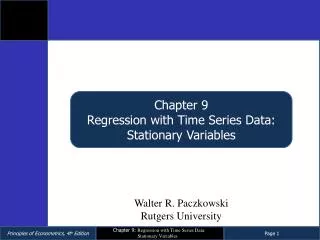
63. We will encounter models with a lagged dependent variable, such as:

65. Suppose we proceed with least squares estimation without recognizing the existence of serially correlated errors. What are the consequences? The least squares estimator is still a linear unbiased estimator, but it is no longer best The formulas for the standard errors usually computed for the least squares estimator are no longer correct Confidence intervals and hypothesis tests that use these standard errors may be misleading

66. It is possible to compute correct standard errors for the least squares estimator: HAC (heteroskedasticity and autocorrelation consistent) standard errors, or Newey-West standard errors These are analogous to the heteroskedasticity consistent standard errors

67. Consider the model yt = �1 + �2xt + et The variance of b2 is: where

68. When the errors are not correlated, cov(et, es) = 0, and the term in square brackets is equal to one. The resulting expression is the one used to find heteroskedasticity-consistent (HC) standard errors When the errors are correlated, the term in square brackets is estimated to obtain HAC standard errors

69. If we call the quantity in square brackets g and its estimate , then the relationship between the two estimated variances is:

70. Let�s reconsider the Phillips Curve model:

71. The t and p-values for testing H0: �2 = 0 are:

72. Return to the Lagrange multiplier test for serially correlated errors where we used the equation: Assume the vt are uncorrelated random errors with zero mean and constant variances:

73. Eq. 9.30 describes a first-order autoregressive model or a first-order autoregressive process for et The term AR(1) model is used as an abbreviation for first-order autoregressive model It is called an autoregressive model because it can be viewed as a regression model It is called first-order because the right-hand-side variable is et lagged one period

74. We assume that: The mean and variance of et are: The covariance term is:

75. The correlation implied by the covariance is:

76. Setting k = 1: ? represents the correlation between two errors that are one period apart It is the first-order autocorrelation for e, sometimes simply called the autocorrelation coefficient It is the population autocorrelation at lag one for a time series that can be described by an AR(1) model r1 is an estimate for ? when we assume a series is AR(1)

77. Each et depends on all past values of the errors vt: For the Phillips Curve, we find for the first five lags: For an AR(1) model, we have:

78. For longer lags, we have:

79. Our model with an AR(1) error is: with -1 < ? < 1 For the vt, we have:

80. With the appropriate substitutions, we get: For the previous period, the error is: Multiplying by ?:

81. Substituting, we get:

82. The coefficient of xt-1 equals -?�2 Although Eq. 9.43 is a linear function of the variables xt , yt-1 and xt-1, it is not a linear function of the parameters (�1, �2, ?) The usual linear least squares formulas cannot be obtained by using calculus to find the values of (�1, �2, ?) that minimize Sv These are nonlinear least squares estimates

83. Our Phillips Curve model assuming AR(1) errors is: Applying nonlinear least squares and presenting the estimates in terms of the original untransformed model, we have:

84. Nonlinear least squares estimation of Eq. 9.43 is equivalent to using an iterative generalized least squares estimator called the Cochrane-Orcutt procedure

85. We have the model: Suppose now that we consider the model: This new notation will be convenient when we discuss a general class of autoregressive distributed lag (ARDL) models Eq. 9.47 is a member of this class

86. Note that Eq. 9.47 is the same as Eq. 9.47 since: Eq. 9.46 is a restricted version of Eq. 9.47 with the restriction d1 = -?1d0 imposed

87. Applying the least squares estimator to Eq. 9.47 using the data for the Phillips curve example yields:

88. The equivalent AR(1) estimates are: These are similar to our other estimates

89. The original economic model for the Phillips Curve was: Re-estimation of the model after omitting DUt-1 yields:

90. In this model inflationary expectations are given by: A 1% rise in the unemployment rate leads to an approximate 0.5% fall in the inflation rate

91. We have described three ways of overcoming the effect of serially correlated errors: Estimate the model using least squares with HAC standard errors Use nonlinear least squares to estimate the model with a lagged x, a lagged y, and the restriction implied by an AR(1) error specification Use least squares to estimate the model with a lagged x and a lagged y, but without the restriction implied by an AR(1) error specification

93. An autoregressive distributed lag (ARDL) model is one that contains both lagged xt�s and lagged yt�s Two examples:

94. An ARDL model can be transformed into one with only lagged x�s which go back into the infinite past: This model is called an infinite distributed lag model

95. Four possible criteria for choosing p and q: Has serial correlation in the errors been eliminated? Are the signs and magnitudes of the estimates consistent with our expectations from economic theory? Are the estimates significantly different from zero, particularly those at the longest lags? What values for p and q minimize information criteria such as the AIC and SC?

96. The Akaike information criterion (AIC) is: where K = p + q + 2 The Schwarz criterion (SC), also known as the Bayes information criterion (BIC), is: Because Kln(T)/T > 2K/T for T = 8, the SC penalizes additional lags more heavily than does the AIC

97. Consider the previously estimated ARDL(1,0) model:

98.

99.

100. For an ARDL(4,0) version of the model:

101. Inflationary expectations are given by:

102.

103. Recall the model for Okun�s Law:

104.

105.

106. Now consider this version:

107. An autoregressive model of order p, denoted AR(p), is given by:

108. Consider a model for growth in real GDP:

109.

110.

112. We consider forecasting using three different models: AR model ARDL model Exponential smoothing model

113. Consider an AR(2) model for real GDP growth: The model to forecast GT+1 is:

114. The growth values for the two most recent quarters are: GT = G2009Q3 = 0.8 GT-1 = G2009Q2 = -0.2 The forecast for G2009Q4 is:

115. For two quarters ahead, the forecast for G2010Q1 is: For three periods out, it is:

116. Summarizing our forecasts: Real GDP growth rates for 2009Q4, 2010Q1, and 2010Q2 are approximately 0.72%, 0.93%, and 0.99%, respectively

117. A 95% interval forecast for j periods into the future is given by: where is the standard error of the forecast error and df is the number of degrees of freedom in the estimation of the AR model

118. The first forecast error, occurring at time T+1, is: Ignoring the error from estimating the coefficients, we get:

119. The forecast error for two periods ahead is: The forecast error for three periods ahead is:

120. Because the vt�s are uncorrelated with constant variance , we can show that:

121.

122. Consider forecasting future unemployment using the Okun�s Law ARDL(1,1): The value of DU in the first post-sample quarter is: But we need a value for GT+1

123. Now consider the change in unemployment Rewrite Eq. 9.70 as: Rearranging:

124. For the purpose of computing point and interval forecasts, the ARDL(1,1) model for a change in unemployment can be written as an ARDL(2,1) model for the level of unemployment This result holds not only for ARDL models where a dependent variable is measured in terms of a change or difference, but also for pure AR models involving such variables

125. Another popular model used for predicting the future value of a variable on the basis of its history is the exponential smoothing method Like forecasting with an AR model, forecasting using exponential smoothing does not utilize information from any other variable

126. One possible forecasting method is to use the average of past information, such as: This forecasting rule is an example of a simple (equally-weighted) moving average model with k = 3

127. Now consider a form in which the weights decline exponentially as the observations get older: We assume that 0 < a < 1 Also, it can be shown that:

128. For forecasting, recognize that: We can simplify to:

129. The value of a can reflect one�s judgment about the relative weight of current information It can be estimated from historical information by obtaining within-sample forecasts: Choosing a that minimizes the sum of squares of the one-step forecast errors:

132. The forecasts for 2009Q4 from each value of a are:

134. Multiplier analysis refers to the effect, and the timing of the effect, of a change in one variable on the outcome of another variable

135. Let�s find multipliers for an ARDL model of the form: We can transform this into an infinite distributed lag model:

136. The multipliers are defined as:

137. The lag operator is defined as: Lagging twice, we have: Or: More generally, we have:

138. Now rewrite our model as:

139. Rearranging terms:

140. Let�s apply this to our Okun�s Law model The model: can be rewritten as:

141. Define the inverse of (1 � ?1L) as (1 � ?1L)-1 such that:

142. Multiply both sides of Eq. 9.82 by (1 � ?1L)-1: Equating this with the infinite distributed lag representation:

143. For Eqs. 9.83 and 9.84 to be identical, it must be true that:

144. Multiply both sides of Eq. 9.85 by (1 � ?1L) to obtain (1 � ?1L)a = d. Note that the lag of a constant that does not change so La = a Now we have:

145. Multiply both sides of Eq. 9.86 by (1 � ?1L):

146. Rewrite Eq. 9.86 as: Equating coefficients of like powers in L yields: and so on

147. We can now find the ߒs using the recursive equations:

148. You can start from the equivalent of Eq. 9.88 which, in its general form, is: Given the values p and q for your ARDL model, you need to multiply out the above expression, and then equate coefficients of like powers in the lag operator

149. For the Okun�s Law model: The impact and delay multipliers for the first four quarters are:

151. We can estimate the total multiplier given by: and the normal growth rate that is needed to maintain a constant rate of unemployment:

152. We can show that: An estimate for a is given by: Therefore, normal growth rate is:

154. AIC criterion AR(1) error AR(p) model ARDL(p,q) model autocorrelation Autoregressive distributed lags autoregressive error autoregressive model BIC criterion correlogram delay multiplier distributed lag weight

156. For the Durbin-Watson test, the hypotheses are: The test statistic is:

157. We can expand the test statistic as:

158. We can now write: If the estimated value of ? is r1 = 0, then the Durbin-Watson statistic d � 2 This is taken as an indication that the model errors are not autocorrelated If the estimate of ? happened to be r1 = 1 then d � 0 A low value for the Durbin-Watson statistic implies that the model errors are correlated, and ? > 0

161. Decision rules, known collectively as the Durbin-Watson bounds test: If d < dLc: reject H0: ? = 0 and accept H1: ? > 0 If d > dUc do not reject H0: ? = 0 If dLc < d < dUc, the test is inconclusive

162. Note that: Further substitution shows that:

163. Repeating the substitution k times and rearranging: If we let k ? 8, then we have:

164. We can now find the properties of et:

165. The covariance for one period apart is:

166. Similarly, the covariance for k periods apart is:

167. We are considering the simple regression model with AR(1) errors: To specify the transformed model we begin with: Rearranging terms:

168. Defining the following transformed variables: Substituting the transformed variables, we get:

169. There are two problems: Because lagged values of yt and xt had to be formed, only (T - 1) new observations were created by the transformation The value of the autoregressive parameter ? is not known

170. For the second problem, we can write Eq. 9C.1 as: For the first problem, note that: and that

171. Or: where

172. To confirm that the variance of e*1 is the same as that of the errors (v2, v3,�, vT), note that: