Download
1 / 24
240 likes | 356 Views
1.2 DESCRIBING DISTRIBUTIONS WITH NUMBERS (Pages 30-46). "If a man stood with one foot in an oven and the other foot in a freezer, statisticians would say that, on the average, he was comfortable." - Quote Magazine , June 29, 1975. 1.2 DESCRIBING DISTRIBUTIONS WITH NUMBERS. OVERVIEW:

E N D
1.2 DESCRIBING DISTRIBUTIONS WITH NUMBERS (Pages 30-46) "If a man stood with one foot in an oven and the other foot in a freezer, statisticians would say that, on the average, he was comfortable." - Quote Magazine, June 29, 1975
1.2 DESCRIBING DISTRIBUTIONS WITH NUMBERS • OVERVIEW: • A numerical summary of a data distribution should somehow indicate its center and its spread. • The concept of spread is important. As a simple example, sets A and B both have a mean of 50. However, the sets are very different in terms of spread. • A = {50,50,50,50,50,50,50,50,50,50} • B = {0,0,0,0,0,100,100,100,100,100}
Measures of center. • Mean (important to understand sigma notation) • Median (the 50th percentile) • Mode (most frequent score. A data set can be multi-modal).
Work 1.24 1.25 1.26 1.27 1.28 1.29 1.30 Read Pages 37 to 42 For next time:
Measures of spread. • Quartiles • Q1 = 25th percentile • Median = 50th percentile • Q3 = 75th percentile • Range (Max. value - min. value) • Interquartile range (Q3 - Q1)
The Five-Number Summary • Minimum • Q1 • Median • Q3 • Maximum • It is very important to note that there are definite conventions for establishing the "big five" for a numerical data set.
You should understand how the values are determined for the following data sets.
Boxplots • The "big five" are all that is needed to construct a boxplot (sometimes called a box-whisker plot) for a data set. • Boxplots are useful when you have lots of data to summarize, where displays like dotplots and stemplots become impractical. • A boxplot does not identify every individual piece of data, but rather summarizes the data by quartiles.
Modified Boxplots • A modified boxplot is frequently used to identify outliers. • An outlier is defined to be a number that is: • more than 1.5 IQRs above Q3 • or less than 1.5 IQRs below Q1 • For example, in Data Set #4 above: • the IQR is 41.1.5 x 41 = 61.5.Q3 + 1.5(IQ Range) = 45 + 61.5 = 106.5. • Since 140 > 106.5, the number 140 is an outlier, and it would be so-identified in a modified boxplot. • The TI-83 produces both types of boxplots.
Important to note: • The mean is greatly influenced by an outlier; the median is not. • The range is greatly influenced by an outlier; the IQR is not. • Q1 and Q3 are not influenced by an outlier.
Work 1.31 1.32 1.33 1.34 Read Pages 43 to 46 For next time:
Statistic vs. Parameter • A statistic is a number that is computed from a sample. • A parameter is a number that is computed from a population. • Means, medians, IQRs, etc. could be statistics or parameters. • Typically Greek letters are used for parameters
Standard Deviation • In statistics, the standard deviation is frequently a very important measure of spread. • The variance is the square of the standard deviation. • There are two different standard deviations, depending on whether it is being computed from a population or from a sample.
Population vs. Sample • A population standard deviation is designated by s, and it is a parameter. • A sample standard deviation is designated by s, and it is a statistic. • s and s are calculated slightly differently • If a data set is large, the difference between s and s very small.
Consider the set W = {10,20,30} The mean of W is 20.
If W is considered to be a population, then the standard deviation and variance are, respectively, s = sqrt(200/3) = 8.16495809 and s2 = 66.6666667. If W is considered to be a sample, then the standard deviation and variance are, respectively, s = sqrt(200/2) = 10 and s2 = 100. Population vs. Sample
Units • It’s significant to note that units attached to a variance are square units. • Whereas, the standard deviation has the same unit as the data itself.
Things to note: • For the present time we will be mostly concerned with the standard deviation, s. • s measures spread about the mean. (The median is not used.) • If s = 0, there is no spread. (In this case, all observations are identical.) • s is influenced by outliers. • s is most meaningful with data that has a symmetrical shape. • If data is heavily skewed, s is not a particularly useful statistic.
Recall the sets A and B described in the OVERVIEW. • Set A has mean = 50, • standard deviation = s = 0, and • variance = s2 = 0 (square units). • Set B has mean = 50, • standard deviation = s = 52.705, and • variance = s2 = 2777.817 (square units).
Degrees of Freedom • The phrase degrees of freedom is mentioned in this section. • This concept will be important in future studies, but for now, an intuitive feeling for the phrase will be provided.
Consider a set of five numbers • Let the sum = 100, thus the mean is 20.
Note that one could replace the four numbers 12, 18, 5, and 43 with any other set of four numbers, and then "adjust" the value of x so that the sum of the five numbers is 100. • That is, four of the numbers can vary freely and, for each set of four numbers, the value x can be "adjusted" to preserve the sum of 100. • In this situation, we say that there are 5-1 = 4 degrees of freedom. • If we had a set of N numbers with a definite sum, then the degrees of freedom would be N-1.
This concludes Chapter 1 • Be sure to look over the Chapter Review on pages 51 to 53. • Note that Question #1 on the 2001 AP Stat exam involved the concept of an outlier and other statistical concepts introduced in Chapter 1. • If you are given a numerical data set, always (I repeat, always) display the shape of the distribution.
Work 1.35 1.36 1.37 Read 1.2 Summary Pages 47 & 48 Chapter 1 Review Pages 51 to 53 Quiz 1.2 next class For next time: