Download
1 / 15
150 likes | 292 Views
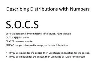
1.2 Describing Distributions with Numbers. Center and spread are the most basic descriptions of what a data set “looks like.” They are intuitively meant to measure exactly what comes to your mind when you hear those terms, but the best way to define them isn’t so obvious.

E N D
Center and spread are the most basic descriptions of what a data set “looks like.” They are intuitively meant to measure exactly what comes to your mind when you hear those terms, but the best way to define them isn’t so obvious. We first investigate center.
Center What is the center? Good question! The most popular measure of center is the mean or average value of a data set. The mean of a data set is computed by summing all data values and then dividing by n. We denote the mean by x. The Greek letter Σ (Sigma) is used as shorthand to mean “sum up.”
Notation • Suppose we are given the data values 10 4 7 12 1 4 10 8. Compute Σx. • We may also combine operations with x and the summation. Compute Σ(x+1). • A nice formula for the mean may then be written as
Problems with mean • Consider the data set 3 2 6 3 5 70 2 4 4 1. Compute the mean of the data. • We have that μ=10, which hardly seems like a good “measure of average.” • The problem can be attributed to the value 70. A value which is considerably larger (or smaller) than the rest of the data pattern is known as an outlier. • Any measure of central tendency that is “sensitive” to extreme values, such as above, is not a resistant measure.
A Resistant Measure • The median for a collection of data values is the number that is exactly in the middle position of the list when the data are arraigned in increasing order. We use M to denote the median. • Let’s find the mean in the example above.
Comparison • The median is a resistant measure of central tendency, unlike the mean, which is a strong advantage. However, the mean takes into account all numerical values while the median only takes the existence of the values into account. • There is a formula for the mean but only a location for the median.
Inadequacies with Centers • What centers do not take into account is the spread of the data. For example, consider the following data sets: A={19 20 20 21} and B={1 20 20 39}. • In both data sets, the mean and median are both 20, but the data of B is much more spread out than the data of A. • Thus, using just a center to describe our data is not good enough. We also need spread.
Measuring spread • The most obvious measure of spread is the range of a set of data; that is, the difference between the highest and lowest data values. The range of a data set is denoted R. • Above, R(A)=21-19=2 and R(B)=39-1=38. • But consider the data set C={1 50 50 50 50 50 50 50 50 50 99} and D={1 10 20 30 40 50 60 70 80 90 99}. Not only are the mean and median in both data sets the same, but so is the range.
Percentile • The mth percentile is the number that separates the bottom m% of the data from the top (100-m)% of the data. It is denoted by PM. • Note that the median of a data set is the 50th percentile so that P50=median.
Quartiles and IQR • We define the first, second, and third quartile by Q1=P25,Q2=P50, and Q3=P75. • The interquartile range, denoted IQR, is defined by IQR=Q3-Q1. • It is easy to convince yourself that IQR is a resistant measure!
The 5 Number Summary • We study a way to present a data set in which the reader can easily read off the quartiles and the high and low values of the data set. • The following is an example of a boxplot. • Min, Q1, M, Q3, Max
E.g. Consider the data set {33, 36, 37, 37 38, 41, 42, 42, 42, 45, 47, 52, 54, 55, 56, 56, 57, 60, 78, 92}. Construct a boxplot. • To identify outliers, we use a modified boxplot. The idea is that instead of drawing the whiskers from Q1 to the lowest value and Q3 to the highest value, we draw the upper whisker from Q3 to the largest data value between Q3 and Q3+1.5xIQR. The lower whisker is drawn from Q1 to the smallest data value between Q1 – 1.5xIQR and Q1. Any data that is not plotted thus far is considered an outlier and is plotted individually. • Construct a modified boxplot for the above data.
Another measure of spread • There are other things we can do. Let’s experiment with the data set 2 3 7 12 on the board. • We have just “discovered” the standard deviation; The standard deviation is denoted by s, and the variance is denoted by s2. They are defined by
Problems and problems Compute the standard deviation for the data sets A and B. “[The standard deviation]… will be large if the observations are widely spread about their mean, and small if the observations are close to their mean.” Unfortunately, none of these measures of dispersion is resistant; that is, they are sensitive to outliers.