Decision Tree Learning

1. Decision Tree Learning ACM Student Chapter, Heritage Institute of Technology 3rd February, 2012 SIGKDD Presentation by SatarupaGuha Sudipto Banerjee AshishBaheti

2. Machine Learning • A computer program is said to learn from experience E with respect to a class of tasks T and performance measure P if its performances at tasks T as measured by P, improves with experience E.

3. An Example: Checkers learning Problem • Task T : Playing checkers • Performance P : Percent of games won by opponents • Experience E : Gained by playing against itself

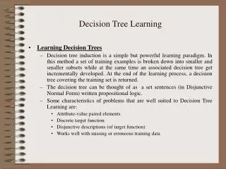
4. Concept Learning Concept learning can be formulated as a problem of searching through a predefined space of potential hypotheses for the hypothesis that best fits the training examples. Much of learning involves acquiring general concepts from specific training examples.

5. Representing Hypotheses • Let H be a hypothesis space. For each h belonging to H, h is a conjunction of literals. • Let X be a set of possible instances each described by a set of attributes. Example- < ?, A2, A3, ?, ?, A6 > • Target function C: X-> {0,1} • Training examples D: positive and negative examples of the target function. <x1, c(x1)> ,…, <xm, c(xm)>

6. Types of Training Examples • Positive Examples: those training examples that satisfy the target function, ie. For which c(x)=1 or TRUE. • Negative Examples: those training examples that do not satisfy the target function, ie. For which c(x)=0 or FALSE.

7. Attribute Types • Nominal / Categorical • Ordinal • Continuous

8. Inductive learning hypothesis • Any hypothesis found to approximate the target function well over a sufficiently large set of training examples, will also approximate the target function well over other unobserved examples. • Any hypothesis h is said to be consistent with a set of training examples D of target concept c iff h(x)=c(x) for each training example <x , c(x)>

9. Classification Techniques • Decision Tree based Methods • Rule-based Methods • Memory based reasoning • Neural Networks • Naïve Bayesand Bayesian Belief Networks • Support Vector Machines

10. Decision Tree • Goal is to create a model that predicts the value of a target variable based on several input variables. 

11. Decision tree representation • Each internal node tests an attribute. • Each branch corresponds to an attribute value. • Each leaf node assigns a classification.

12. A quick recap • CNF = Conjunctive Normal Form • DNF = Disjunctive Normal Form

13. Disjunctive NormalForm • In Boolean Algebra, a formula is in DNF if it is a disjunction of clauses, where a clause is a conjunction of literals. Also known as Sum of Products. • Example: (A ^ B ^ C) V (B ^ C)

14. Conjunctive Normal Form • In Boolean Algebra, a formula is in CNF if it is a conjunction of clauses, where a clause is a disjunction of literals. Also known as Product of Sum. • Example: (A V B V C) ^ (B V C)

15. Decision Tree: contd. • Decision trees represent a disjunction(OR) of conjunctions(AND) of constraints on the attribute values of instances, • Each path from the tree root to a leaf corresponds to a conjunction of attribute tests, and the tree itself to a disjunction of these conjunctions. • Hence, DT represents a DNF.

16. Attribute splitting • 2- way split • Multi- way split

17. CarType Family Luxury Sports CarType CarType {Sports, Luxury} {Family, Luxury} {Family} {Sports} Splitting Based on Nominal Attributes • Multi-way split: Use as many partitions as distinct values. • Binary split: Divides values into two subsets. Need to find optimal partitioning. OR

18. Size Small Large Medium Size Size {Small, Medium} {Medium, Large} {Large} {Small} Splitting Based on Ordinal Attributes • Multi-way split: Use as many partitions as distinct values. • Binary split: Divides values into two subsets. Need to find optimal partitioning. OR

19. Splitting Based on Continuous Attributes

20. categorical categorical continuous class Example of a Decision Tree Splitting Attributes Refund Yes No NO MarSt Married Single, Divorced TaxInc NO < 80K > 80K YES NO Model: Decision Tree Training Data

21. DT Classification Task

22. Measures of Node Impurity • Entropy • GINI Index • Misclassification Error

23. Entropy • It characterizes the impurity of an arbitrary collection of examples. It is a measure of randomness. Entropy(S)= -p log p - p log p Where , S is a collection containing positive & negative examples of some target concept. P is the proportion of positive ex in S. P is the proportion of negative ex in S.

24. An example of Entropy • Let S is a collection of 14 examples, including 9 positive & 5 negative examples, denoted by [9+, 5-]. • Then entropy[9+, 5-] = -9/14 log(9/14) – 5/14 log(5/14) = 0.94

25. More on Entropy • In a more general sense, Entropy = 0, if all members belong to the same class. = 1, if collection contains equal no. of positive & negative examples. = lies between 0 & 1, if there are unequal no. of positive & negative examples.

26. GINI Index • GINI Index for a given node t : • (NOTE: p( j | t) is the relative frequency of class j at node t). • Maximum (1 - 1/nc) when records are equally distributed among all classes, • implying least interesting information • Minimum (0.0) when all records belong to one class, • implying most interesting information

27. Examples for computing GINI P(C1) = 0/6 = 0 P(C2) = 6/6 = 1 Gini = 1 – (0)^2 – (1)^2 = 1-0-1= 1 P(C1) = 1/6 P(C2) = 5/6 Gini = 1 – (1/6)^2 – (5/6)^2 = 0.278 P(C1) = 2/6 P(C2) = 4/6 Gini = 1 – (2/6)^2 – (4/6)^2 =0.444

28. Splitting Based on GINI • When a node p is split into k partitions (children), the quality of split is computed as, where, ni = number of records at child i, n = number of records at node p.

29. Binary Attributes: Computing GINI Index • Splits into two partitions • Effect of Weighing partitions: • Larger and Purer Partitions are sought for. B? Yes No Node N1 Node N2 GINI(N1) = 1 – (5/7)2 – (2/7)2= 0.408 GINI (N2) = 1 – (1/5)2 – (4/5)2= 0.320 GINI (Children) = 7/12 * 0.408+ 5/12 * 0.320= 0.371

30. Categorical Attributes: Computing Gini Index • For each distinct value, gather counts for each class in the dataset • Use the count matrix to make decisions Two-way split (find best partition of values) Multi-way split

31. A set of training examples Day outlook humidity wind play tennis D1 sunny high weak no D2 sunny high strong no D3 overcast high weak yes D4 rain high weak yes D5 rain normal weak yes D6 rain normal strong no D7 overcast normal strong yes D8 sunny high weak no D9 sunny normal weak yes D10 rain normal weak yes

32. Decision Tree Learning Algorithms • Variations of a core algorithm that employs a top-down, greedy search through the space of possible decision trees. • Examples are Hunt’s Algorithm, CART, ID3, C4.5, SLIQ,SPRINT, Mars.

33. Algorithm ID3

34. Algorithm ID3 • Greedy algorithm that grows the tree top-down. • Begins with the question "which attribute should be tested at the root of the tree?” • A statistical property called information gain is used.

35. Information Gain • Expected reduction in entropy caused by partitioning the example according to a particular attribute. • Gain of an attribute A relative to a collection of example S is defined as- Gain(S,A)= Entropy(S) - ∑ |Sv|/|S| Entropy(Sv) v->Values(A) where Values(A): set of all positive values of an attribute A. Sv: subset of S for which attribute A has value v.

36. Information Gain: contd. • Gain(S,A) is the information provided about the target function value, given the value of some other attribute A. • Example: S is a collection described by attributes including Wind, which can have the values Weak or Strong. Assume S has 14 examples. • Then S=[9+, 5-] S weak= [6+, 2-] S strong= [3+, 3-]

37. Information Gain: contd. • Gain(S, wind) = Entropy(S) – (8/14) Entropy(S weak) – (6/14) Entropy(S strong) = 0.94 – (8/14) 0.811 = 0.048

38. Play Tennis example: revisited Day outlook humidity wind play tennis D1 sunny high weak no D2 sunny high strong no D3 overcast high weak yes D4 rain high weak yes D5 rain normal weak yes D6 rain normal strong no D7 overcast normal strong yes D8 sunny high weak no D9 sunny normal weak yes D10 rain normal weak yes

39. Application of ID3 on Play Tennis • There are 3 attributes- Outlook, humidity and Wind • We need to choose one of them as the root of the tree. We make this choice based on the information gain(IG) of each of the attributes. The one with the highest IG gets to be the root. • The calculations are shown in the following slides.

40. Quick recap of formulae • Entropy: p log (1/p ) + p log ( 1/p ) • Information Gain: Gain(S,A)= Entropy(S) - ∑ |Sv|/|S| Entropy(Sv) v->Values(A) Where S is the collection, A is a particular attribute. Values(A): set of all positive values of an attribute A. Sv: subset of S for which attribute A has value v.

41. Calculations: • For Outlook: • The training set has 6 positive and 4 negative examples. Hence entropy =4/10* lg(10/4) + 6/10* lg(10/6)= 0.970 • Outlook can have 3 values- sunny [ 1+, 3- ] rain [ 3+, 1- ] overcast.[ 1+ ] Entropy of sunny= ¼ * lg 4 + ¾* lg (4/3) =0.324 Entropy of rain = ¾ * lg (4/3) + ¼ * lg 4 =0.324 Entropy of overcast= 2/4* lg (2/2) =0

42. Calculations: • Sv/S for each of them are as follows: sunny- 4/10 (means 4 out of 10 examples have sunny as their outlook) rain - 4/10 overcast- 2/10 • Hence, Information gain of outlook = 0.970–( 4/10 *0.324*2 + 2/10*0) = 0.711

43. Calculations: • For Humidity: • The training set has 6 positive and 4 negative examples. Hence entropy = 0.970 • Humidity can take 2 values- High [3+,2-] Normal [4+, 1-] • Entropy of High = 3/5* lg (5/3) + 2/5* lg (5/2) = 0.970 • Entropy of Normal = 1/5* lg 5 + 4/5* lg(5/4) = 0.7195

44. Calculations: • Sv/S for High = 5/10 for normal = 5/10 Hence IG( Humidity) =0.970 – (5/10*0.970 + 5/10*0.7195) =0.125 • Similarly for Wind, the IG is 0.0910. • Hence, IG(Outlook)=0.7110 IG(Humidity)=0.125 IG(Wind)= 0.0910 • Comparing the IG s of the 3 attributes, we find Outlook has got the highest IG(0.7110)

45. Partially formed tree • Hence outlook is chosen as the root of the decision tree. • The partially formed decision tree is as follows: Outlook Sunny [1+,3-] Rain [3+,1-] Overcast[2+] yes

46. Further calculations: • Since sunny and rain have both positive and negative examples, they have fair degrees of randomness and hence need to be classified further. • For sunny : As computed earlier, Entropy of sunny= 0.324 • Now, we need to find the corresponding humidity and wind for those training examples who have outlook=sunny.

47. Further calculations Day Outlook Humidity wind Play tennis D1 sunny high weak no D2 sunny high strong no D8 sunny high weak no D9 sunny normal weak yes For Humidity: Sv/S* Entropy(high)= ¾*0=0 Sv/S* Entropy(low)=1/4*0=0

48. Calculations: • Zero because there is no randomness. All the examples that have Humidity= high have Play tennis= No and those having Humidity=low have Play Tennis=yes. • IG (S sunny, Humidity)= 0.324- 0 = 0.324 • For Wind: • Sv/S * Entropy(weak)=¾*(2/3*lg 3/2) + 1/3*lg 3=0.687. Sv/S* Entropy(strong)=1/4* 0=0 • IG(S sunny, Wind) = 0.324 – 0.687 = -0.363 • Clearly, humidity has a higher IG.

49. Outlook Sunny[1+,3-] Rain[3+,1-] Humidity Overcast[2+] High[3+] Normal[1+] yes No yes

50. Further Calculations • Now for Rain[ 3+,1-], Day Outlook Humidity Wind Play tennis D4 Rain high weak yes D5 Rain normal weak yes D6 Rain normal strong no D10 Rain normal weak yes