Ch 3. Decision Tree Learning

1. Ch 3. Decision Tree Learning • Decision trees • Basic learning algorithm (ID3) • Entropy, information gain • Hypothesis space • Inductive bias • Occam’s razor in general • Overfitting problem & extensions • post-pruning • real values, missing values, attribute costs, …

2. Decision Tree for PlayTennis Outlook Sunny Overcast Rain Humidity Yes Wind High Normal Strong Weak No Yes No Yes

3. Training Examples

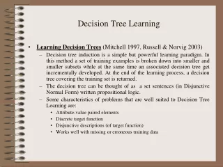
4. Decision Tree Learning • Classify instances • sorting them down the tree to a leaf node containing the class (value) • based on attributes of instances • branch for each value • Widely used, practical method of approximating discrete-valued functions • Robust to noisy data !! • Capable of learning disjunctive expressions • Typical bias: prefer smaller trees

5. Each internal node tests an attribute Each branch corresponds to an attribute value node Each leaf node assigns a classification Decision Tree for PlayTennis Outlook Sunny Overcast Rain Humidity High Normal No Yes

6. No Outlook Sunny Overcast Rain Humidity Yes Wind High Normal Strong Weak No Yes No Yes Decision Tree for PlayTennis Outlook Temperature Humidity Wind PlayTennis Sunny Hot High Weak ?

7. Decision Tree for Conjunction Outlook=Sunny  Wind=Weak Outlook Sunny Overcast Rain Wind No No Strong Weak No Yes

8. Decision Tree for Disjunction Outlook=Sunny  Wind=Weak Outlook Sunny Overcast Rain Yes Wind Wind Strong Weak Strong Weak No Yes No Yes

9. Decision Tree for XOR Outlook=Sunny XOR Wind=Weak Outlook Sunny Overcast Rain Wind Wind Wind Strong Weak Strong Weak Strong Weak Yes No No Yes No Yes

10. Outlook Sunny Overcast Rain Humidity Yes Wind High Normal Strong Weak No Yes No Yes Decision Tree • decision trees represent disjunctions of conjunctions (Outlook=Sunny  Humidity=Normal)  (Outlook=Overcast)  (Outlook=Rain  Wind=Weak)

11. When to use Decision Trees? • Instances presented as attribute-value pairs • Target function has discrete values • classification problems • Disjunctive descriptions required • disjunction of conjunctions of constraints on attribute values of instances • Training data may contain • errors • missing attribute values • Examples: • Medical diagnosis • Credit risk analysis • Object classification for robot manipulator

12. Top-Down Induction of Decision Trees -ID3 • A  the “best” decision attribute for next node • Assign A as decision attribute for node • For each value of A create new descendant • Sort training examples to leaf nodes according to the attribute value of the branch • If all training examples are perfectly classified (same value of target attribute) stop, else iterate over newleaf nodes.

13. [29+,35-] A1=? A2=? [29+,35-] True False True False [18+, 33-] [21+, 5-] [8+, 30-] [11+, 2-] Which Attribute is ”best”?

14. Entropy • S is a sample of training examples • p+ is the proportion of positive examples • p- is the proportion of negative examples • Entropy measures the impurity of S Entropy(S) = -p+ log2 p+ - p- log2 p-

15. Entropy • Entropy(S)= expected number of bits needed to encode class (+ or -) of randomly drawn members of S (under the optimal, shortest length-code) • Why? • Information theory optimal length code assign –log2 p bits to messages having probability p. • So the expected number of bits to encode (+ or -) of random member of S: -p+ log2 p+ - p- log2 p-

16. [29+,35-] A1=? A2=? [29+,35-] True False True False [18+, 33-] [21+, 5-] [8+, 30-] [11+, 2-] Information Gain • Gain(S,A): expected reduction in entropy due to sorting S on attribute A Gain(S,A)=Entropy(S) - vvalues(A) |Sv|/|S| Entropy(Sv) Entropy([29+,35-]) = -29/64 log2 29/64 – 35/64 log2 35/64 = 0.99

17. [29+,35-] A1=? A2=? [29+,35-] True False True False [18+, 33-] [21+, 5-] [8+, 30-] [11+, 2-] Information Gain Entropy([21+,5-]) = 0.71 Entropy([8+,30-]) = 0.74 Gain(S,A1)=Entropy(S) -26/64*Entropy([21+,5-]) -38/64*Entropy([8+,30-]) =0.27 Entropy([18+,33-]) = 0.94 Entropy([8+,30-]) = 0.62 Gain(S,A2)=Entropy(S) -51/64*Entropy([18+,33-]) -13/64*Entropy([11+,2-]) =0.12

18. Training Examples

19. Selecting the Best Attribute S=[9+,5-] E=0.940 S=[9+,5-] E=0.940 Humidity Wind High Normal Weak Strong [3+, 4-] [6+, 1-] [6+, 2-] [3+, 3-] E=0.592 E=0.811 E=1.0 E=0.985 Gain(S,Wind) =0.940-(8/14)*0.811 – (6/14)*1.0 =0.048 Gain(S,Humidity) =0.940-(7/14)*0.985 – (7/14)*0.592 =0.151

20. Selecting the Best Attribute S=[9+,5-] E=0.940 Outlook Over cast Rain Sunny [3+, 2-] [2+, 3-] [4+, 0] E=0.971 E=0.971 E=0.0 Gain(S,Outlook) =0.940-(5/14)*0.971 -(4/14)*0.0 – (5/14)*0.971 =0.247

21. ID3 Algorithm [D1,D2,…,D14] [9+,5-] Outlook Sunny Overcast Rain Ssunny=[D1,D2,D8,D9,D11] [2+,3-] [D3,D7,D12,D13] [4+,0-] [D4,D5,D6,D10,D14] [3+,2-] Yes ? ? Gain(Ssunny , Humidity)=0.970-(3/5)0.0 – 2/5(0.0) = 0.970 Gain(Ssunny , Temp.)=0.970-(2/5)0.0 –2/5(1.0)-(1/5)0.0 = 0.570 Gain(Ssunny , Wind)=0.970= -(2/5)1.0 – 3/5(0.918) = 0.019

22. ID3 Algorithm Outlook Sunny Overcast Rain Humidity Yes Wind [D3,D7,D12,D13] High Normal Strong Weak No Yes No Yes [D6,D14] [D4,D5,D10] [D8,D9,D11] [D1,D2]

23. + - + A1 A2 + - + + - + - - + + - - Hypothesis Space Search ID3 A2 A2 - - + - + A3 A4 + - - +

24. Hypothesis Space Search ID3 • Hypothesis space is complete! • Target function surely in there… • Outputs a single hypothesis • No backtracking on selected attributes (greedy search) • Local minimal (suboptimal splits) • Statistically-based search choices • Robust to noisy data • Inductive bias (search bias) • Prefer shorter trees over longer ones • Place high info. gain attributes close to the root

25. Inductive Bias in ID3 • H is the power set of instances X • Unbiased ? • Preference for short trees, and for those with high information gain attributes near the root • Bias is a preference for some hypotheses, rather than a restriction of the hypothesis space H • Compare bias to C-E • ID3: complete space, incomplete search --> bias from search strategy • C-E: incomplete space, complete search --> bias from expressive power of H

26. Occam’s Razor • Why prefer short hypotheses? • Argument in favor: • Fewer short hypotheses than long hypotheses • A short hypothesis that fits the data is unlikely to be a coincidence • A long hypothesis that fits the data might be a coincidence • Argument against: • There are many ways to define small sets of hypotheses • E.g. All trees with a prime number of nodes that use attributes beginning with ”Z” • What is so special about small sets based on size of hypothesis???

27. Overfitting - definition • Consider error of hypothesis h over • Training data: errortrain(h) • Entire distribution D of data: errorD(h) • Hypothesis hH overfits training data if there is an alternative hypothesis h’H such that errortrain(h) < errortrain(h’) and errorD(h) > errorD(h’) • Possible reasons: noise and small samples • coincidences possible with small samples • noisy data creates a large tree h • h’ not fitting it is likely to work better

28. Overfitting in Decision Trees error validation set training set optimal #nodes #nodes

29. Avoid Overfitting How can we avoid overfitting? • Stop growing when data split not statistically significant • Grow full tree then post-prune • has been found more successful • Minimum description length (MDL): Minimize: size(tree) + size(misclassifications(tree))

30. How to decide tree size? • What criterion to use • separate test set to evaluate the use of pruning • use all data, apply statistical test to estimate if expanding/pruning is likely to produce improvement • use an explicit complexity measure (coding length of data & tree), stop growth when minimized

31. Training/validation sets • Available data split • training set: apply learning to this • validation set: evaluate result • accuracy • impact of pruning • ‘safety check’ against overfit • common strategy: 2/3 for training

32. Reduced error pruning • Pruning • make an inner node a leaf node • assign it the most common class • Procedure Split data into training and validation set Do until further pruning is harmful: 1. Evaluate impact on validation set of pruning each possible node (plus those below it) 2. Greedily remove the one that most improves the validation set accuracy • Produces smallest version of most accurate subtreee

33. Rule Post-Pruning • Procedure (C4.5 uses a variant) • infer DT as usual (allow overfit) • convert tree to rules (one per path) • prune each rule independently • remove preconditions if result is more accurate • sort rules by estimated accuracy into a desired sequence to use • apply rules in this order in classification

34. Rule post-pruning… • Estimating the accuracy • separate validation set • training data & pessimistic estimates • data is too favorable for the rules • compute accuracy & standard deviation • take lower bound from given confidence level (e.g. 95%) as the measure • very close to observed one for large sets • not statistically valid but works

35. Why convert to rules? • Distinguishing different contexts in which a node is used • separate pruning decision for each path • No difference for root/inner • no bookkeeping on how to reorganize tree if root node is pruned • Improves readability

36. Outlook Sunny Overcast Rain Humidity Yes Wind High Normal Strong Weak No Yes No Yes Converting a Tree to Rules R1: If (Outlook=Sunny)  (Humidity=High) Then PlayTennis=No R2: If (Outlook=Sunny)  (Humidity=Normal) Then PlayTennis=Yes R3: If (Outlook=Overcast) Then PlayTennis=Yes R4: If (Outlook=Rain)  (Wind=Strong) Then PlayTennis=No R5: If (Outlook=Rain)  (Wind=Weak) Then PlayTennis=Yes

37. Continuous values • Define new discrete-valued attr • partition the continuous value into a discrete set of intervals • Ac = true iff A < c • How to select best c? (inf. gain) • Example case • sort examples by continuous value • identify borderlines

38. Continuous values… • Fact • value maximizing inf. gain lies on such boundary • Evaluation • compute gain for each boundary • Extensions • multiple values • LTUs based on many attributes

39. Alternative selection measures • Information gain measure favors attributes with many values • separates data into small subsets • high gain, poor prediction • E.g.: Imagine using Date=xx.yy.zz as attribute • perfectly splits the data into subsets of size 1 • Use gain ratio instead of information gain!! • penalize gain with split information • sensitive to how broadly & uniformly attribute splits data • Entropy of S with respect to values of A • earlier: entropy of S w.r.t target values

40. Split information • GainRatio(S,A) = Gain(S,A) / SplitInfo (S,A) • SplitInfo(S,A) = -i=1..c |Si|/|S| log2 |Si|/|S| • Where Si is the subset for which attribute A has the value vi • Discourages selection of attr with • many uniformly distr. Values • n values: log n, boolean: 1 • Better to apply heuristics to select attributes • compute Gain first • compute GR only when Gain large enough (above average)

41. Another alternative • Distance-based measure • define a metric between partitions of the data • evaluate attributes: distance between created & perfect partition • choose the attribute with closest one • Shown • not biased towards attr. with large value sets • Many alternatives like this in the literature.

42. Missing values • Estimate value • other examples with known value • Compute Gain(S,A), A(x) unknown • assign most common value in S • most common with class c(x) • assign probability for each value, distribute fractionals of x down • Similar techniques in classification

43. Attributes with differing costs • Measuring attribute costs something • prefer cheap ones if possible • use costly ones only if good gain • introduce cost term in selection measure • no guarantee in finding optimum, but give bias towards cheapest • Replace Gain by : Gain2(S,A)/Cost(A) • Example applications • robot & sonar: time required to position • medical diagnosis: cost of a laboratory test

44. Summary • Decision-tree induction is a popular approach to classification that enables us to interpret the output hypothesis • Practical learning method • discrete-valued functions • ID3: top-down greedy algorithm • Complete hypothesis space • Preference bias - shorter trees preferred. • Overfitting is an important issue • Reduced error pruning • Rule post-pruning • Techniques exist to deal with continuous attributes and missing attribute values.