Download
1 / 40
430 likes | 602 Views
Overview and Rationale for Modelica Stream Connectors January 27, 2009. Revisions:. Contents. Part A Overview 1. Stream Variables and Stream Operators 2. Modeling with Streams Part B Rationale 3. Basic Problems of Fluid Connectors 4. Stream Connection Semantics

E N D
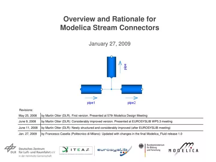
Overview and Rationale forModelica Stream Connectors January 27, 2009 Revisions:
Contents Part A Overview 1. Stream Variables and Stream Operators 2. Modeling with Streams Part B Rationale 3. Basic Problems of Fluid Connectors 4. Stream Connection Semantics 5. Reliable Handling of Ideal Mixing 6. Open Issues 7. Status 8. History and Contributors
Part A Overview At the 57th Modelica design meeting (May 25-28, 2008) a new fundamental type of connector variables "stream" was introduced for the nextModelica Language Specification Version 3.1, because the two standard types of port variables used in all component oriented modeling systems potential/flow, across/through, effort/flow variables are not sufficient to model flow of matter in a reliable way. Modelica_Fluid 1.0 is based on this new concept. These slides give an introduction in to this new connector type and provide a rationale why it is introduced and the benefits of the concept.
1. Stream Variables and Stream Operators Purpose • Reliable handling of convective mass and energy transport inthermo-fluid systems with bi-directional flow of matter. • Relevant boundary conditions and balance equations are fulfilled in a connection point. (convective) transport of matter mass and energy balance fulfilledin the idealized connection point
Examples of an interface for fluid components { • A stream variable hi of a connector i is associated with • a flow variable m_flow ("0 = Σ m_flowi") and • a stream balance equation ("0 = Σm_flowi*<upstream value of hi>")
inStream(h2) h2 h3 inStream(h3) h1 inStream(h1) Reliable handling of bi-directional flow: (mixing value for m_flowi > 0)
Example of a volume – pressure drop network volume volume pressure drop pressure drop inStream(h6) h1 inStream(h4) h5 inStream(h2) h3 inStream(h1) h6 inStream(h5) inStream(h3) h4 h2 inStream(h1) = h2 = inStream(h3) = h4 = inStream(h5) = h6inStream(h6) = h5 = inStream(h4) = h3 = inStream(h2) = h1 Energy balance in volume 1: der(U1) = m_flow1*actualStream(h1) = m_flow1*(if m_flow1 > 0 theninStream(h1) else h1) = m_flow1*(if m_flow1 > 0 then h6else h1)
2. Modeling with Streams Connector definition: connector FluidPort SI = Modelica.SIunits; SI.AbsolutePressure p "Pressure in connection"; flow SI.MassFlowRate m_flow "Mass flow rate"; stream SI.SpecificEnthalpy h_outflow "h if m_flow <= 0"; stream SI.MassFraction X_outflow[nX] "X if m_flow <= 0"; end FluidPort; If a connector has one or more stream variables, exactly one (scalar) flow variable must be present which is the flow associated with all stream variables. Modeling with stream variables is very simple (see following examples)! For notational convenience, the equations for the mass fractions X are not shown in the following examples.
Example: Mixing Volume model MixingVolume "Volume that mixes two flows" replaceable package Medium = Modelica.Media.Interfaces.PartialMedium; FluidPort port_a, port_b; parameter Modelica.SIunits.Volume V "Volume of device"; Modelica.SIunits.Mass m "Mass in device"; Modelica.SIunits.Energy U "Inner energy in device"; Medium.BaseProperties medium(preferredMediumStates=true); equation // Definition of port variables port_a.p = medium.p; port_b.p = medium.p; port_a.h_outflow = medium.h; port_b.h_outflow = medium.h; // Mass and energy balance m = V*medium.d; U = m*medium.u; der(m) = port_a.m_flow + port_b.m_flow; der(U) = port_a.m_flow*actualStream(port_a.h_outflow) + port_b.m_flow*actualStream(port_b.h_outflow); end MixingVolume;
Example: Isenthalpic fluid transport model IsenthalpicFlow "No energy storage/losses, e.g. pressure drop, valve, ..." replaceable package Medium=Modelica.Media.Interfaces.PartialMedium; FluidPort port_a, port_b: Medium.ThermodynamicState port_a_state_inflow "State at port_a if inflowing"; Medium.ThermodynamicState port_b_state_inflow "State at port_b if inflowing"; equation // Medium states for inflowing fluid port_a_state_inflow = Medium.setState_phX(port_a.p, inStream(port_a.h_outflow)); port_b_state_inflow = Medium.setState_phX(port_b.p, inStream(port_b.h_outflow)); // Mass balance 0 = port_a.m_flow + port_b.m_flow; // Instantaneous propagation of enthalpy flow between the ports with // isenthalpic state transformation (no storage and no loss of energy) port_a.h_outflow = inStream(port_b.h_outflow); port_b.h_outflow = inStream(port_a.h_outflow); // (Regularized) Momentum balance port_a.m_flow = f(port_a.p, port_b.p,Medium.density(port_a_state_inflow), Medium.density(port_b_state_inflow)); end IsenthalpicFlow;
Example: Isentropic fluid transport model IsenthalpicFlow "No energy storage, e.g. pump, heat losses, ..." replaceable package Medium = Modelica.Media.Interfaces.PartialMedium; FluidPort port_a, port_b: Medium.ThermodynamicState port_a_state_inflow "State at port_a if inflowing"; Medium.ThermodynamicState port_b_state_inflow "State at port_b if inflowing"; Modelica.SIunit.Power P_ext "Energy flow via other connectors" equation // Medium states for inflowing fluid port_a_state_inflow = Medium.setState_phX(port_a.p, inStream(port_a.h_outflow)); port_b_state_inflow = Medium.setState_phX(port_b.p, inStream(port_b.h_outflow)); // Mass balance 0 = port_a.m_flow + port_b.m_flow; // Instantaneous propagation of enthalpy flow between the ports with // isentropic state transformation port_a.h_outflow = Medium.isentropicEnthalpy(port_a.p,inStream(port_b.h_outflow)); port_b.h_outflow = Medium.isentropicEnthalpy(port_b.p,inStream(port_a.h_outflow)); // Energy balanced to compute energy flow exchanged with other ports 0 = P_ext + port_a.m_flow*actualStream(port_a.h_outflow) + port_b.m_flow*actualStream(port_b.h_outflow); // (Regularized) Momentum balance port_a.m_flow = f(port_a.p, port_b.p, Medium.density(port_a_state_inflow), Medium.density(port_b_state_inflow)); end IsenthalpicFlow;
Example: Temperature sensor model TemperatureSensor "Ideal temperature sensor" replaceable package Medium = Modelica.Media.Interfaces.PartialMedium; FluidPort port(m_flow(min=0)); // No flow out of sensor ever Modelica.Blocks.Interfaces.RealOutput T "Upstream temperature"; equation T = Medium.temperature(Medium.setState_phX(port.p, inStream(port.h_outflow)); port.m_flow = 0; port.h_outflow = Medium.specificEnthalpy(Medium.setState_pTX( Medium.reference_p, Medium.reference_T)); // This value will never be used, since m_flow(min=0), // but it will show up in the plot window. end TemperatureSensor; Setting "m_flow.min=0" is very important, in order that the temperature sensor hasno influence on the stream that it measures, if all mass flow rates are zero; since then "max(-port.m_flow,ε) = 0" in the inStream(..)-operators of the connected ports!!!
Example: Infinite Reservoir model FixedBoundary_pT "Infinite reservoir with fixed pressure and temperature" replaceable package Medium = Modelica.Media.Interfaces.PartialMedium; FluidPort port; parameter Medium.AbsolutePressure p "Boundary pressure"; parameter Medium.Temperature T "Boundary temperature"; equation port.p = p; port.h_outflow = Medium.specificEnthalpy(Medium.setState_pTX(p, T)); end FixedBoundary_pT;
provide a rationale, why reliable bi-directional flow modelingrequires a third type of connector variable (streams), discusses details of the connection semantics of streams, shows why stream connectors lead to reliable models. Part B Rationale The following slides
3. Basic Problems of Fluid Connectors Desired connector for bi-directional flow of matter. The intensive quantitiestransported with the matter (like h) have the newly introduced "stream" prefix: connector FluidPort import SI = Modelica.SIunits; SI.AbsolutePressure p "Pressure in connection point"; flow SI.MassFlowRate m_flow "Mass flow rate"; stream SI.SpecificEnthalpy h "Specific enthalpy"; end FluidPort; Observation This is the most simplest connector description form for the desired class of models(independently how the connected components are described, e.g. lumped,discretized PDE, PDE, ...). It is very unlikely that a "simpler" connector exists. Goal Define connection semantic of stream variables, so that the balance equationsfor stream variables in an infinitesimal small connection point are fulfilled andthe equations can be solved reliably.
Central Question: What is the meaning of a stream variable, such as "h"? Balance equations of stream variables for 3 connected components(independently how the components are described, e.g. lumped, PDE, ...) m2.h m1.m_flow m1.h m3.h h_mix (1) 0 = m1.m_flow*(if m1.m_flow > 0 then h_mix else m1.h) + m2.m_flow*(if m2.m_flow > 0 then h_mix else m2.h) + m3.m_flow*(if m3.m_flow > 0 then h_mix else m3.h) (2) 0 = m1.m_flow + m2.m_flow + m3.m_flow From the balance equations, it seems natural that the stream variables are oneof the occurring variables, e.g., h_mix or m1.h
but: then, the result will be of the form: h_mix = if m1.m_flow > 0 then ... else ...m1.h = if m1.m_flow > 0 then ... else ... e.g. for 2 connected components: h_mix = if m1.m_flow > 0 then m2.h else m1.h this means that m1,h, m2.h, h_mix etc. are computed by equations that contain if-clauses which depend on the mass flow rate. If algebraic systems of equations occur (due to initialization, or ideal mixing,or pressure drop components directly connected together etc.), then these equation systems, inevitably, have unknowns that depend on the unknown mass flow direction, i.e., nasty non-linear equation systems occur that are difficult to solve (since Boolean unknowns as iteration variables)!!!
The issue appears even in the most simple case of MixingVolume – PressureDrop – MixingVolume connection, if the mass flow rate in the pressure drop does not only depend on pressure, but also on density as a function of the medium state: mixing volume mixing volume pressure drop h1,p1 h4,p4 h2,p1 h3,p4 m_flow h2 = if m_flow > 0 then h4 else h1 h3 = h2; // !!!!! d2 = f1(p1,h2) // density d3 = f1(p4,h3) m_flow = f2(p1, p4, d2, d3) Note: Even for the most simplest case (volume – pressure drop – volume), a nasty non-linear equation system appears, since m_flow = f2(..., m_flow > 0);Can sometimes be fixed by replacing "m_flow > 0" with "p4 - p1 > 0"
Additionally, every pressure drop component is not differentiableat m_flow = 0. If non-linear equation systems occur, then this system isnot differentiable at a critical point, and then every non-linear solver has difficulties. mixing volume mixing volume pressure drop h1,p1 h4,p4 h2,p1 h3,p4 m_flow h2 = if m_flow > 0 then h4 else h1 h3 = h2; // !!!!! d2 = f1(p1,h2) // density d3 = f1(p4,h3) m_flow = f2(p1, p4, d2, d3) Major problem: Independently of the flow direction:h3 = h2 m_flow > 0: m_flow = f2(..., d2(p1,h4), d3(p4,h4)); m_flow < 0: m_flow = f2(..., d2(p1,h1), d3(p4,h1)); However (see next slides): f2(..) must be a function of d2(p1,h1), d3(p1,h4) !!!
When m_flow > 0, dp > 0: The "blue" curve (m_flow1) is computed.When m_flow < 0, dp < 0: The "red" curve (m_flow2) is computed. When m_flow changes from positive to negative, the interpolation jumps from curve "blue" to "red". This means, that m_flow is not differentiable at m_flow = 0. If m_flow appears in a non-linear equation system, this is not good, because thepre-requisite of a non-linear solver is not fulfilled in the critical point at m_flow = 0!!!! d(p1,h4) d(p1,h1)
Correct treatment: m_flow = f2(..) is a function of d2(p1,h1), d3(p1,h4) !!! d(p1,h4) d(p1,h1) In order that the correct f2(..) function is used ("green" curve), the "density" of the "actual" flow (m_flow > 0) and the "density" of the "reversed flow" (m_flow < 0) are neededat the same time instant. Only then, regularization around m_flow = 0is possible, leading to a smooth characteristic.
Summary: It is impossible to arrive at reliable, bi-directional flow models, if the actual intensive quantities (like h_mix, h1, h2, ...) are used in the connector equations. mixing volume mixing volume pressure drop h1,p1 h4,p4 h2,p1 h3,p4 m_flow Note, the only way to avoid the identified problems is to not computeh_mix, m1.h, etc. Instead: d2_outflow = f1(p1,h4) // flow from h4 to h1 d3_outflow = f1(p4,h1) // flow from h1 to h4 m_flow = f2(p1, p4, d2_outflow, d3_outflow)
4. Stream Connection Semantics • Central idea: • compute value for "outflow" and • inquire value for "inflow" with operator "inStream(..)" port_a.h_outflow inStream(port_a.h_outflow) port_a.h_outflow port_b.h_outflow inStream(port_b.h_outflow) instream(port_a.h_outflow
pipe1.port_a.p = pipe2.port_a.ppipe1.port_a.p = pipe3.port_a.p0 = pipe1.port_a.m_flow + pipe2.port_a.m_flow + pipe3.port_a.m_flow Basic connector definition connector FluidPort SI = Modelica.SIunits; SI.AbsolutePressure p "Pressure in connection point"; flow SI.MassFlowRate m_flow "Mass flow rate"; stream SI.SpecificEnthalpy h_outflow "h close to port if m_flow < 0"; end FluidPort; connect(pipe1.port_a, pipe2.port_b);connect(pipe1.port_a, pipe3.port_b); pipe3.port_a.m_flow No connection equations are generated for stream variables (!) pipe1.port_a.m_flow pipe2.port_a.m_flow pipe1.port_a.h_outflow
(1) 0 = max(m1.c.m_flow,0)*h_mix - max(-m1.c.m_flow,0)*m1.c.h_outflow + max(m2.c.m_flow,0)*h_mix – max(-m2.c.m_flow,0)*m2.c.h_outflow + max(m3.c.m_flow,0)*h_mix – max(-m3.c.m_flow,0)*m3.c.h_outflow (2) 0 = max( m1.c.m_flow,0) + max( m2.c.m_flow,0) + max(m3.c.m_flow,0) - max(-m1.c.m_flow,0) – max(-m2.c.m_flow,0) – max(m3.c.m_flow,0) m3 m1 m2 c.h_outflow h_mix(h for ideal mixing) (3) h_mix = (max(-m1.c.m_flow,0)*m1.c.h_outflow +max(-m2.c.m_flow,0)*m2.c.h_outflow +max(-m3.c.m_flow,0)*m3.c.h_outflow) / (max(m1.c.m_flow,0) +max(m2.c.m_flow,0) +max(m3.c.m_flow,0)) mass balance (4) h_mix = (max(-m1.c.m_flow,0)*m1.c.h_outflow + max(-m2.c.m_flow,0)*m2.c.h_outflow + max(-m3.c.m_flow,0)*m3.c.h_outflow) / (max(-m1.c.m_flow,0) + max(-m2.c.m_flow,0) +max(-m3.c.m_flow,0)) balance equations model : m1,m2,m3;connector: c;flow : m_flow stream : h_outflow (1) 0 = m1.c.m_flow*(if m1.c.m_flow > 0 then h_mix else m1.c.h_outflow) + m2.c.m_flow*(if m2.c.m_flow > 0 then h_mix else m2.c.h_outflow) + m3.c.m_flow*(if m3.c.m_flow > 0 then h_mix else m3.c.h_outflow) (2) 0 = m1.c.m_flow + m2.c.m_flow + m3.c.m_flow
(4) h_mix = (max(-m1.c.m_flow,0)*m1.c.h_outflow + max(-m2.c.m_flow,0)*m2.c.h_outflow + max(-m3.c.m_flow,0)*m3.c.h_outflow) / (max(-m1.c.m_flow,0) + max(-m2.c.m_flow,0) +max(-m3.c.m_flow,0)) Definition: inStream(m1.c.h_outflow) = h_mix for m1.c.m_flow > 0 Reason: This definition prepares for the changing flow direction at m1.c.m_flow = 0:If only m1.c.m_flow is changing the flow direction, thenh_mix is discontinuous at m1.c.m_flow = 0. However,h_mix for m1.c.m_flow > 0 is continuous at m1.c.m_flow = 0 since m1.c.h_outflow does not appear in the equation, because for inflowing flow, this variable does not influence the mixing andthe same formula is used also for the reversed direction!!!
For 2 connections: (6) inStream(m1.c.h_outflow) = (max(-m2.c.m_flow,0)*m2.c.h_outflow / max(-m2.c.m_flow,0) = m2.c.h_outflow For 3 connections with m3.c.m_flow.min=0 (One-Port Sensor): (7) inStream(m1.c.h_outflow) = m2.c.h_outflow (8) inSteram(m3.c.h_outflow) = (max(-m1.c.m_flow,0)*m1.c.h_outflow + max(-m2.c.m_flow,0)*m2.c.h_outflow) / (max(-m1.c.m_flow,0) + max(-m2.c.m_flow, 0)) (4) h_mix = (max(-m1.c.m_flow,0)*m1.c.h_outflow + max(-m2.c.m_flow,0)*m2.c.h_outflow + max(-m3.c.m_flow,0)*m3.c.h_outflow) / (max(-m1.c.m_flow,0) + max(-m2.c.m_flow,0) +max(-m3.c.m_flow,0)) Definition: inStream(m1.c.h_outflow) = h_mix for m1.c.m_flow > 0 (5) inStream(m1.c.h_outflow) = (max(-m2.c.m_flow,0)*m2.c.h_outflow + max(-m3.c.m_flow,0)*m3.c.h_outflow) / (max(-m2.c.m_flow,0) + max(-m3.c.m_flow, 0)) ≈ (max(-m2.c.m_flow,ε)*m2.c.h_outflow + max(-m3.c.m_flow,ε)*m3.c.h_outflow) / (max(-m2.c.m_flow,ε) + max(-m3.c.m_flow,ε))
If all mass flow rates are zero, the stream balance equation is identicallyfulfilled, independently of the values of h_mix, and mi.c.h_outflow. Therefore, there are an infinite number of solutions. The basic idea is to approximate the "max(..)" function to avoid this case: (5) inStream(m1.c.h_outflow) = (max(-m2.c.m_flow,0)*m2.c.h_outflow + max(-m3.c.m_flow,0)*m3.c.h_outflow) / (max(-m2.c.m_flow,0) + max(-m3.c.m_flow, 0)) ≈ (max(-m2.c.m_flow,ε)*m2.c.h_outflow + max(-m3.c.m_flow,ε)*m3.c.h_outflow) / (max(-m2.c.m_flow,ε) + max(-m3.c.m_flow,ε)) Then a unique solution of this equation always exists. If all mass flow rates are identically to zero, the result is the mean value of the involved specific enthalpies: (6) inStream(m1.c.h_outflow) ≈ (max(-m2.c.m_flow,ε)*m2.c.h_outflow + max(-m3.c.m_flow,ε)*m3.c.h_outflow) / (max(-m2.c.m_flow,ε) + max(-m3.c.m_flow,ε)) = (ε*m2.c.h_outflow + ε*m3.c.h_outflow) / (ε + ε) = (m2.c.h_outflow + m3.c.h_outflow) / 2
The actual regularization is a bit more involved, in order that • an approximation is only used, if all mass flow rates are small, • the characteristic is continuous and differentiable(max(.., ε) is continuous but not differentiable) // Actual regularization for small mass flow rates // Determine denominator s for exact computation s := sum( max(-mj.c.m_flow,0) ) // Define a "small number" eps (nominal(v) is the nominal value of v) eps := relativeTolerance*min(nominal(mj.c.m_flow)) // Define a smooth curve, such that alpha(s>=eps)=1 and alpha(s<=0)=0// (using a polynomial of 3rd order) alpha := smooth(1, if s > eps then 1 else if s > 0 then (s/eps)^2*(3-2*(s/eps)) else 0); // Define function positiveMax(v) as a linear combination of max(v,0)// and of eps along alpha positiveMax(-mj.c.m_flow) := alpha*max(-mj.c.m_flow,0) + (1-alpha)*eps; // Use "positiveMax(..)" instead of "max(.., eps)" in the// inStream(..) definition!
5. Reliable Handling of Ideal Mixing reference problem • "DryAirNasa" (ideal gas with f(p,T)) and"FlueGasSixComponents" (mixture of ideal gases with 6 substances) • Detailed pipe friction correlations for the laminar and turbulent flow regimes • Ideal mixing point (no volume) in the connection point. All the details are described in a report from M. Sielemann and M. Otter.Only the major results are presented on the following slides.
(Note: with a volume in the connection point there would be 2+6=8 state variables, i.e., an implicit DAE solverwould have 8 iteration variables). Number of iteration variablesfor"FlueGasSixComponents"(mixture of ideal gases with 6 substances)
Basic (previous) form of "pressure drop" component: replaceable package Medium = Modelica.Media.Interfaces.PartialMedium; Medium.BaseProperties medium_a_inflow; Medium.BaseProperties medium_b_inflow;equation medium_a_inflow.p = port_a.p; medium_b_inflow.p = port_b.p; medium_a_inflow.h = inStream(port_a.h_outflow); medium_b_inflow.h = inStream(port_b.h_outflow); port_a.h_inflow = medium_a_inflow.h; port_b.h_inflow = medium_b_inflow.h; port_a_d_inflow = medium_a_inflow_d; port_b_d_inflow = medium_b_inflow_d;; If medium is not f(p.h), a non-linear equation system appears, in order to computemedium_a_inflow.h from medium_a_inflow.T (and from the pressure).For an ideal mixing point (or any other non-linear equation system), a tool willtherefore select T as iteration variable.
Severe disadvantage: Temperature is discontinuous and therefore theiteration variable is discontinuous!!! T as iteration variable(discontinuous)-> at m_flow = 0, jumpin iteration variable;every non-linear solverhas difficulties with this. m_flow asiteration variable(continuous)
New form of "pressure drop" component: replaceable package Medium = Modelica.Media.Interfaces.PartialMedium; equation port_a.h_outflow = inStream(port_b.h_outflow); port_b.h_outflow = inStream(port_a.h_outflow); port_a_state_inflow = Medium.setState_phX( port_a.p, inStream(port_a.h_outflow),...); port_b_state_inflow = Medium.setState_phX( port_b.p, inStream(port_b.h_outflow),...); port_a_inflow = Medium.density(port_a_state_inflow); port_b_inflow = Medium.density(port_b_state_inflow); If medium is not f(p.h), no (explicit) non-linear equation system appears, since themedium state is computed from the known port properties. However, the function "setState_phX" solves internally a non-linear equation system(with Brents algorithm; a fast and very reliable algorithm to solve one non-linearalgebraic equation in one unknown).
A tool can now compute all variables in a point with N connections from N-1 mass flow rates and 1 pressure in an explicit forward sequence and therefore selects these variablesas iteration variables (and these variables are always continuous): • The N-th mass flow rate is computed from the mass balance • The port-specific mixing enthalpies (h_mix(m_flow_i = 0)) can be computed, since they depend only on known variables(enthalpies in the volumes and the mass flow rates). • The medium states can be computed via Medium.setState_phX(..),since p,h,X are known now. • All medium properties can be computed from the medium state, especially the density. • Via the momentum balance, the mass flow rates can be computed(= residue equations). Analysis does also hold for initialization: With this approach, initialization willwork much better, since mass flow rates are selected as iteration variables.A default start value of zero for mass flow rates is often sufficient for the solver.
Summary If the "streams" concept is used, and the pressure drop components are implemented as sketched in the previous slide, then an ideal mixing point with N connections gives rise to a non-linear system of algebraic equations(if N > 2 and no min-attributes are set) that has the following properties: • The number of iteration variables is N (independent of the medium, and how many substances are in the medium). • The iteration variables are continuous everywhere(since as iteration variables, N-1 mass flow rates and one pressure is used). • The iteration variables are in most cases differentiable(due to the definition of stream-variables and of the inStream(..) operator).The iteration variables are not differentiable, if all mass flow rates in an ideal mixing point become zero at the same time instant.If this is not the case, they are differentiable. • Default start values of zero for the mass flow rates and for the pressure drop in the pressure drop components, are good guess values for theiteration variables (independent of the medium). It can therefore be expected that a solution of the equation system is easyto compute by every reasonable non-linear equation solver.
6. Open Issues • For a regular network of the usual "Volume – Pressure Drop – Volume" structure a non-linear algebraic equation in one unknown is present for every connector of a pressure drop component, if the medium states arenot p,h,X. It seems possible to remove all these equation systems by clever symbolic analysis. This issue is not critical, because these scalar implicit equations can be solved reliably. The only issue is to enhance efficiency. • If components from discretized PDEs are connected together, there are two options with respect to the mathematical structure. • One option is to split the momentum balance between two components in two parts, leading to two half-momentum-balances on either side of the connection. This results in one non-linear algebraic equation in one unknown (the pressure) for every connection point, which can be numerically troublesome, expecially at initialization. • The other option is to split the mass and energy balances in two parts, leading to two half-mass-balances on either side of the connection. This results in a high-index problem. If the tool can handle the index reduction, the resulting equations can be solved reliably • Both options are available in the DistributedPipe model of Modelica_Fluid
7. Status • Detailed specification text for Modelica 3.1 available • (Positive) voting for the specification text for inclusion in Modelica 3.1 • Fully functional implementation in Dymola available (version 7.1 and later) • Work going on to implement the concept in OpenModelica and MathModelica • Final release of Modelica_Fluid library v.1.0 changed to new connector design • Detailed tests with sandbox libraries by Rüdiger Franke and Michael Sielemann • All examples of Modelica_Fluid simulate without problems • Initialization parameters removed from all pressure drop coefficients(no longer needed, since m_flow used as iteration variable; default of m_flow.start = 0 is a good guess value; a better one can be provided via a parameter) • Plan: Tests in EUROSYSLIB with larger and realistic benchmarks.
The tool requirements for "stream" support is very modest: • No special symbolic transformation algorithms needed! • Connection semantic is trivial:Generate no connection equation for stream variables • The inStream(..) operator requires to analyze all corresponding stream-variables in a connection set (e.g. with respect to "min(..)" attributes).A tool could decide to only support 1:1 connections in the beginning.The inStream(..) operator is then trivial to implement. • Inside/outside connections (= hierarchical connections) complicate issues a bit (similarly to flow-variables), but nothing serious
8. History and Contributors • 2002:ThermoPower connectors by Francesco Casella(this is the basis of the stream connector concept) • 2002: First version of Modelica_Fluid that is refined until 2008.Many basic concepts are from Hilding Elmqvist.It was never possible to make the library reliable. • Jan. 2008: upstream(..) operator by Hilding Elmqvist(triggered the further development) • Jan. 2008: new formulation of "ideal mixing" from Francesco Casella(this is the basis of the inStream(..) operator) • March 2008: proposal of "stream" connectors by Rüdiger Franke • April 2008: refined proposal by Rüdiger Franke & Martin Otter,prototype in Dymola by Sven Erik Mattsson,improved definition of inside/outside connector by Hans Olsson,test of the concept by Rüdiger Franke and Michael Sielemann,reformulation to improve the numerics by M. Sielemann and M. Otter,transformation of Modelica_Fluid to streams by M. Otter • May 2008: final proposal developed by Modelica fluid group at the57th design meeting and (positive) vote for inclusion in Modelica 3.1. • Jan 2009: Modelica_Fluid 1.0 released, based on stream connectors