Download
1 / 16
160 likes | 302 Views
Quantized Hall effect. Experimental systems. MOSFET’s (metal-oxide-semiconductor-field-effect-transistor.) Two-dimensional electron gas on the “capacitor plates” which can move laterally. Experimental systems.

E N D
Experimental systems • MOSFET’s (metal-oxide-semiconductor-field-effect-transistor.) • Two-dimensional electron gas on the “capacitor plates” which can move laterally.
Experimental systems • GaAs heterostructures: higher mobility. 2D electron gas confined to the interface of the heterostructures because of the band offset.
Experimental results • RH: xy • R: xx • Integer vs fractional QHE.
Experiment was done under a high magnetic field • The energy of the 2D electrons are quantized under a large magnetic field. The density of states is illustrated on the right. There are gaps between the Landau levels.
Topics to be covered: • Physics of MOSFET’s • Landau levels • Transport. (We address this first.)
Relationship between conductivity and resistivity • Ji=jijEj; Ei=jijJj. • xx=yy/ [xxyy-xy2]. When ii=0 in between the Landau levels, ii=0 also! • xy=-xy/ [xxyy-xy2] remains finite even when ii=0.
Conductivity ,= 0% dv eiu< [j(u),j(0)]>/+ in0e2,/m
Hall conductivity x,y= 0% dt ei t [< a|jx(t)|b><b|jy(0)|a>-<a| jy(0)|b><b|jx(t )|a>] [fa-fb] / < a|jx(t)|b>=<a|eitHjxe-itH|b> =<a|eitEajxe-itEb|b> = eit(Ea-Eb) <a|jx|b> x,y= 0% dt ei t [eit(Ea-Eb) < a|jx|b><b|jy|a>- eit(Eb-Ea) <a| jy|b><b|jx|a>] [fa-fb] / x,y=i [< a|jx|b><b|jy|a>/(+ Ea-Eb) - <a| jy|b><b|jx|a>/(+ Eb-Ea)] [fa-fb] /
Hall conductivity • Zero frequency limit, L’Hopital’s rule, differentiate numerator and denominator with respect to , get x,y=i [< a|jx|b><b|jy|a> - <a| jy|b><b|jx|a>] [fa-fb] /( Ea-Eb)2
Topological consideration • J= i ki/m (=1, e=1), H=i ki2/2m+V(r ); • Jx= H/ kx x,y=i dk [< a| H/ kx|b><b| H/ ky |a> - <a| H/ ky|b><b| H/ kx|a>] [fa-fb]/ /( Ea-Eb)2 Perturbation theory: |a> =j |j><j| H|a> /(Ej-Ea) ; for a change in wave vector k, H= k( H/ k). Hence |a>/ kx =j |j><j| H/ kx|a>/(Ej-Ea);
Hall conductivity • x,y=idkdr [ ( a*( r)/ kx)(a(r)/ ky ) - (a*(r)| / ky)(a (r)/ kx ) ] f(a). The above contain contributions with both |a> and |b> occupied but those contributions cancel out. • From Stokes’s theorem, the volume integral in k can be converted to a surface integral:
Hall conductivity • Stokes: d2 k k x g = s d k .g . Consider g = *k. • x,y=i dr sdk . k*( r) k(r)/k . The surface integral is over the perimeter of the Brillouin zone. • This expression is also called the Berry phase in previous textbook. • Let =u exp(i). Then =[ u+u i ] ei. Now dr * = dr u2 =1. Hence dr uk u=0. dr *k = dr u2 i k.
Topological Invariant • In general (r+a)=exp(ika)(r). At the zone boundary, Ga=. Exp(iGa)=-1 is real. At the zone boundary, the phase is not a function of r. x,y=i, dk . dru2 i k/k =- dk . k/k =2 n. • Crucial issues are that n need not be zero; the electrons are not localized.
Substitute (3) into (1). LHS =E. RHS=(E-t+i<n|R[n(R)]>t R). • We thus get -t+i<n|R[n(R)]>t R=0. • x,y=i dk .[ dr k*( r) k(r)/k.] The quantity in the square bracket corresponds to a Berry phase. k is the parameter is this case.