Download
1 / 67
690 likes | 1.2k Views
Random Walk on Graphs and its Algorithmic Applications. Shengyu Zhang Winter School, ITCSC@CUHK, 2009. Random walk on graphs. On an undirected graph G: Starting from vertex v 0 Repeat for a number of steps: Go to a random neighbor. Simple but powerful. Road map: Random walk. Parameters

E N D
Random Walk on Graphs and its Algorithmic Applications Shengyu Zhang Winter School, ITCSC@CUHK, 2009
Random walk on graphs On an undirected graph G: • Starting from vertex v0 • Repeat for a number of steps: • Go to a random neighbor. • Simple but powerful.
Road map: Random walk Parameters /Properties Algorithms • k-SAT • st-connectivity Hitting time • PageRank • Approximate counting • Error-reduction Mixing time
Road map: Quantum walk Short intro to math model of quantum mechanics Types Algorithms Element Distinctness Discrete QW Formula Evaluation Continuous QW
PART I. Random Walk Key parameter 1: Hitting time
Hitting time • Recall the process of random walk on a graph G. • Starting vertex v0 • Repeat for a number of steps: • Go to a random neighbor. • Hitting time: H(i,j) = expected time to visit j (for the first time), starting at i j i
0 1 2 … n-1 i j (n/2)-line (n/2)-complete graph Undirected graphs • Complete graph • H(i,j) = n-1 (i≠j) • Line: • H(i,j) = j2-i2 (i<j) • In particular, H(0,n-1) = (n-1)2. • General graph: • H(i,j) = O(n3).
k-SAT: satisfiability of k-CNF formula • n variables x1, …, xn∊{0,1} • m clauses, each being OR of k literals • Literal: xi or ¬xi • e.g. (k=3): (¬x1)٧x5 ٧x7 • 3-CNF formula: AND of these m clauses • e.g. ((¬x1)٧x5 ٧x7)٨(x2 ٧(¬x5)٧ (¬x7))٨(x1 ٧x7 ٧x8) • 3-SAT Problem: Given a 3CNF formula, decide whether there is an assignment of variables s.t. the formula evaluates to 1. • For the above example, Yes: x5=1, x7=0, x1=1
P vs. NP • P: problems that can be easily solved • “easily”: in polynomial time • NP: problems that can be easily verified. • Formally: ∃ a polynomial time verifier V, s.t. for any input x, • If the answer is YES, then ∃y s.t. V(x,y) = 1 • If the answer is NO, then ∀y, V(x,y) = 1 • The question of TCS: Is P = NP? • Intuitively, no. NP should be much larger. • It’s much easier to verify (with help) than to solve (by yourself) • mathematical proof, appreciation of good music/food, … • Formal proof? We don’t know yet. • One of the 7 Millennium Problems by CMI.① ① http://www.claymath.org/millennium/P_vs_NP/
NP-completeness • k-SAT is NP-complete, for any k ≥ 3. • NP-complete: • In NP • All other problems in NP can be reduced to it in poly. time • NP-complete problems are the hardest ones in NP. • 3-SAT is in NP: • witness --- satisfying assignment A • Verification: evaluate formula with variables assigned by A • [Cook-Levin] 3-SAT is NP-complete.
How about 2-SAT? • While 3-SAT is the hardest in NP, 2-SAT is solvable in polynomial time. • Here we present a very simple randomized algorithm, which has polynomial expected running time.
Algorithm for 2-SAT • 2SAT: each clause has two variables/negations • Alg [Papadimitriou]: • Pick any assignment • Repeat O(n2) time • If all satisfied, done • Else • Pick any unsatisfied clause • Pick one of the two literals each with ½ probability, and flip the assignment on that variable (x1∨x2)∧(x2∨¬x3) ∧(¬x4∨x3) ∧(x5∨x1) x1, x2, x3, x4, x5 0, 1, 0, 1, 0 1
Analysis • (x1∨x2)∧(x2∨¬x3) ∧(¬x4∨x3) ∧(x5∨x1) • x1, x2, x3, x4, x5 • 0, 1, 0, 1, 0 • If unsatisfiable: never find an satisfying assignment • If satisfiable, there exists a satisfying assignment x • If our initially picked assignment x’ is satisfying, then done. • Otherwise, for any unsatisfied clause, at least one of the two variables is assigned a value different than that in x • Randomly picking one of the two variables and flipping its value increases # correct assignments by 1 w.p. ≥ ½
Analysis (continued) • Consider a line of n+1 points, where k represents “we’ve assigned k variables correctly” • “correctly”: the same way as x • Last slide: Randomly picking one of the two variables and flipping its value increases # correct assignments by 1 w.p. ≥ ½ • Thus the algorithm is actually a random walk on the line of n+1 points, with Pr[going right] ≥ ½. • Hitting time (i → n): O(n2) • So by repeating this flipping process O(n2) steps, we’ll reach x with high probability.
st-Connectivity • Problem: Given a graph G and two vertices s and t on it, decide whether they are connected. • BFS/DFS (starting at s) solves the problem in linear time. • But uses linear space as well. • Question: Can we use much less space?
Simple random walk algorithm • A randomized algorithm takes O(log n) space. • Starting at s, perform the random walk for O(n3) steps. If ever see t, output YES and stop. • output NO. • Why it works? H(s,t) = O(n3). • If s can reach t, then we should see it within O(n3) time.
Convergence • Now let’s study the probability distribution of the particle after a long time. • What do we observe? • The distribution converges touniform… • wherever it starts. • Q: Does this hold in general? v u w
v1 v2 v3 v4 v5 v1 v2 v3 v4 v5 v6 Convergence • Well, Yes and No. • Consider the following cases • on undirected graphs. • Case 1: The graph is unconnected. • Case 2: The graph is bipartite. • [Thm] For any connectednon-bipartite graph, and any starting point, the random walk converges.
v u w Converges to what? • In the previous triangle example: uniform. • In general? • As a result of the convergence, the distribution doesn’t change by the matrix • If the particle is on the graph according to the distribution, then further random walk will result in the same distribution. • We call it the stationary distribution. • [Fact] It’s unique.
stationary distribution • [Fact] It’s the following distribution: π(v) = d(v)/2m • d(v) = degree of v, i.e. # of neighbors. • m: |E|, i.e. # of edges. • [Proof] Consider one step of walk: π’(v) = ∑u: (u,v)∊E p(u)∙[1/d(u)] = ∑u: (u,v)∊E [d(u)/2m]∙[1/d(u)] = ∑u: (u,v)∊E 1/2m = d(v)/2m = π(v) So π is the stationary distribution. • For regular graphs, π is the uniform distribution.
Proportional to degree • Note: the stationary distribution π(v) = d(v)/2mis proportional to the degree of v. • What’s the intuition? The more neighbors you have, the more chance you’ll be reached. • We will see another natural interpretation shortly.
Speed of the convergence • We’ve seen that random walk converges to the stationary distribution. • Next question: how fast is the convergence? • Let’s define the mixing time as min {T: ∥pi(T) - π∥ ≤ε}where pi(T): the distribution in time T, starting at i.∥∙∥: some norm. • We’ll see the reason of mixing later. Now let’s first see an example you run into everyday.
PageRank • Google gives each webpage a number for its “importance”. • [IT] Google: 10, Microsoft: 9, Apple: 9 • [Media] NYTimes: 9, CNN: 10, sohu: 8, newsmth: 7 • [Sports] NBA: 7, CBA: 7, CFA: 7 • [University] MIT: 9, CUHK: 8, … … Tsinghua, Pku, Fudan, IIT(B): 9 • When you search for something by making a query, a large number of related webpages are retrieved. • What webpages to retrieve? Information Retrieval. That’s an orthogonal issue.
Ranking • How to give this big corpus to you? • Search engines rank them based on the “importance”, and give them in descending order. • Thus presumably the first page contains the 10 most important webpages related to your query. • Question: How to rank? • PageRank: Use the vast link structure as in indicator of an individual page’s value.
Reference system • Webpage A has a link to webpage B A thinks B is useful. • Think of it as A writing a recommendation letter for B. • So a webpage with a lot of other pages pointing to it is probably important. • A guy getting a lot of letters is strong. • Further, pointers from pages that are themselves important bear more weight. • Letters by Noga, László, Sasha, Avi, Andy, … mean a lot. • But the importance of those pages also need to be calculated… we have a recurrence equation.
Furthermore • If page A has a lot of links, then each link means less. • Ok, you get Einstein’s letter, but you know what, last year everyone on the market got his letter. • So let’s assume that page A’s reference weight is divided evenly to all pages B that A links to. • Recurrence equation: R(A) = ∑B: B→A R(B)/d(B)where d(B) = # pages C that B links to
Sink issue • R(A) = ∑B: B→A R(B)/d(B) has a problem. • There are some “sink” pages that contain no links to other pages. • Sinks accumulate weights without giving out. • The recurrence equation only has solutions with weight on sinks, losing the original intension of indicating the importance of all pages. • To handle this, we modify the recursion:R(A) = (1-α)/N + α∑B: B→A R(B)/d(B) • Force each page to have a (1- α)-fraction of weights (evenly) going to all pages. • So each A also receives a weight of (1- α)/N from all pages • α: around 0.85
Random Walk view • Note that the recursion R(A) = (1-α)/N + α∑B: B→A R(B)/d(B) is exactly the random walk on the graph, where at each point A, we • w/ prob. α, follow a random link; • w/ prob. (1-α), go to a random page. • Question: How to solve this recurrence equation? • # webpages: ~ 30 billion (and counting…)
Algorithm • Recall: the random walk converges to the stationary distribution! • It’s a bit different since it’s random walk on directed graphs, but this PageRank matrix has all good properties we need so that the random walk also converges to the solution. • Algorithm: start from any distribution, run a few iterations of random walk, and output the result. • Google: 50-100 iterations, need a few days. • That should be close to the stationary distribution, which serves as indictor of the importance of pages.
Next • We’ll see a bit math behind the mixing story.
Mathematics behind the mixing • [Eigenvalue decomposition] A symmetric matrix MNN can be written as M = ∑i=1,…,nλiξiξiT • λi: eigenvalue. Order them: |λ1| ≥ |λ2| ≥ |λ3| ≥ … ≥ |λn| • ξi: (column) eigenvector, i.e. Mξi = λiξi • The eigenvectors are orthonormal. • ∥ξi∥2=1 • ξi, ξj = 0, for all i≠j • M2 = (∑i=1,…,nλiξiξiT)(∑j=1,…,nλjξjξjT) = ∑i,jλiξiξiT λjξjξjT = ∑i,jλi λj ξi,ξi ξjξjT = ∑iλi2ξjξiT • Mt = ∑iλitξjξiT
Random walk in matrix form • A: adjacency matrix. (Aij = 1 if (i,j) ∊E; 0 o.w.) • P: probability transition matrix. • Pij = 1/di if (i,j) ∊E; 0 o.w. • P = D-1A, where D = diag(d1, …, dn). (di: deg(i)) • For any distribution p, PTp is the distribution after one step of random walk • N = D-1/2AD-1/2 = D1/2PD-1/2 • Nij = 1/(didj)1/2 if (i,j) ∊E; 0 o.w. • N is symmetric, so N can be written as N = ∑i=1,…,nλiξiξiT • Random Walk for t steps: • Pt = (D-1/2ND1/2)t = D-1/2NtD1/2 = D-1/2 (∑iλitξiξiT)D1/2= ∑iλitD-1/2ξiξiTD1/2
Why mixing? Why to π? • [Thm] For connected non-bipartite graph, N has • λ1 = 1 and ξ1 = π1/2 = ((d1/2m)1/2, …, (dn/2m)1/2) is the square root version of the stationary distribution (so that the l2 norm is 1). • |λ2| < 1. (So is all other λi’s.) • Random Walk for t steps: Pt = ∑i λitD-1/2ξiξiTD1/2 • First item: λ1tD-1/2ξ1ξ1TD1/2 = D-1/2(1/2m)[(didj)1/2]ijD1/2= (1/2m)[dj]ij • For any starting distribution p, (1/2m)[dj]ijTp = π.
Speed of the convergence • All other items: since |λi|<1, λitD-1/2ξiξiTD1/2→0! • Speed of convergence depends on how close |λ2| is to 1. • PageRank matrix: |λ2| = α (≈ 0.85) • Expander: 1-|λ2| = Ω(1)
The rest of the talk • Only ideas are given. • Many details are omitted. • I may cheat a bit to illustrate the main steps.
Algorithm 4: Approximately counting • Task: estimate the size of an exponentially large set V • Example: Given G, count # of perfect matchings. • Approach: find a chain V0⊆V1⊆…⊆Vm=V • |V0| is easy to compute; • m = poly(n) layers; • Each ratio |Vi+1|/|Vi| = poly(n) is easy to estimate. • Then |V| = |V0| (|V1|/|V0|) (|V2|/|V1|)… (|Vn|/|Vn-1|) can be estimated. • Question: How to estimate |Vi+1|/|Vi|?
Estimate the ratio • Estimate by random sampling: • Generate a random element uniformly distributed in Vi+1, see how often it hits Vi. • Question: How to uniformly sample Vi+1? • By random walk • We construct a regular graph with vertex set Vi+1 • The algorithm runs efficiently (i.e. in poly(n) time) if the walk converges to uniform rapidly (i.e. in poly(n) time). • It’s the case in perfect matching counting problem.
Error reduction • Task: Reduce the error of a randomized algorithm A. • Error: Prr∈{0,1}^m[r is bad for A] = 1/3 → ε? • Naïve approach: • Draw k random strings r1, …, rk, • Run algorithm A using r1, …, rk and get k answers • Output the majority of the answers • [Fact] the error drops to 2-Θ(k) . --- Chernoff’s bound • Randomness complexity: mk. • Question: Can we reduce the error prob w/o using too many additional random bits? B {0,1}m
Expander graph • Expander:Eigenvalue gap is large --- Ω(1) • Random walk converges very fast --- O(log n). • Highly connected --- diameter O(log n) • Large boundary --- any subset has lots of edges going out • Could be sparse --- ∃ constant degree expanders. • We know how to construct them explicitly.
Algorithm for error reduction • New Algorithm A’: • Construct an expander with V = {0,1}m • Start from a random vertex r1 • Perform a random walk (r1, r2,…, rk) of length k • Random algorithm A using r1, r2,…, rk and get k answers • Output the majority of the answers • Thm: the error prob of A’ is also 2-Θ(k) • How many random bits used? m + O(k) • The expander is of constant degree. • Highly dependent! Why it works? B {0,1}m
Expander: large boundary • For simplicity, consider the one-side error case: • Algorithm A’ wrong ↔ Whole walk in B. • Expander: Every set has a large boundary. • At every step, it walks outside B w.p. Ω(1). • Pr[k steps never out] = 2-Θ(k) Non-expander {0,1}m: all random strings B Boundary
1 1 |1 |1 0 0 |0 |0 Quantum mechanics in one slide Physics Math | 1 α|0+β|1 (|α|2+|β|2=1) β Physical System Unit Vector α,β: amplitudes | 0 α Evolution Unitary Matrix A classical bit Measurement Projection A quantum bit (qubit) Composition Tensor Product Measure by |0and|1: - get 0 w.p. |α|2; system →|0; - get 1 w.p. |β|2; system →|1. State space for 2 bits: all combinations {00, 01, 10, 11} Classical: State space for 2 qubits: the space span{|00,|01,|10,|11} Quantum:
Quantum walk • Many things become quite tricky. • Even the definition of quantum walk. • We’ll ignore the formal definitions here, but only present some results.